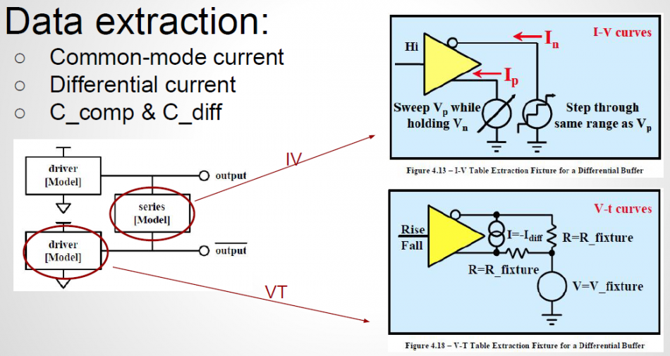
Flow considerations:
Two major considerations when developing a modeling flow are consistency and flexibility. This is particular true when it comes to differential buffer modeling. As discussed in our previous post, a half/true differential buffer goes through most of the same steps as single ended buffer yet certain process must be elaborated (e.g. modeling of the 2d surface sweep) and order needs to be preserved (i.e. extract C_Diff, I_Diff before performing VT simulation). In this post, we will briefly discuss how these considerations are incorporated into design concepts and realized in our SPIBPro modeling flow.
Design setup:
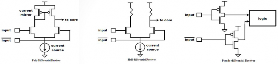
Conceptually, user does not need to know whether a buffer is true/half/pseudo differential before modeling. The IBIS cookbook V4 also states this and also use encrypted hspice as an example… as it’s black box and can’t be deciphered, a model developer needs to assume coupling exists between P and N (thus true differential). The computed differential current from both 2D sweeps of IV and C_Diff will reveal whether such (true differential) assumption is valid. The decision can then be made based on the value of current.. if it’s in uA or nA range, then coupling is insignificant and can be modeled as pseudo differential.
In reality, we may argue that one should start with pseudo-differential approach and switch to half/full differential only if the final validation suggest so. This is because modeling engineer usually can get insights about buffer to be modeled by talking to the circuit designer (usually in the same company, also no needs to reveal or know much of the design details during such inquiry). In addition, the DC sweep of extra dimension and modelings of the half/true differential flow are often overkill for many of the designs.
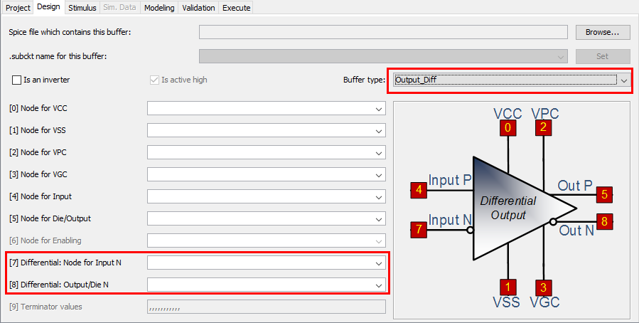
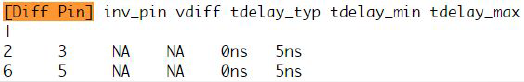
In terms of modeling setup, only input and output (for N pin) are needed in addition to common single-ended buffer. A model type selection of “differential” is sufficient to indicate the differential modeling flow rather than linear single-ended modeling.
Modeling flow overview:
The modeling flow is summarized in the picture below: the key change here is that flow is not linear anymore. The simulation and post-processing stages need to be gone through twice. When simulating for the first time, only IV/C_Die sweep are needed. The data is then post-process for the first time to extract the common-mode and differential-mode current. The latter will also be modeled as a separated component in this stage. This differential component is then inserted between P and N pins in the transient netlist and simulated in the second iteration of the simulation step. However, only VT data is needed this time. When that’s done, all IV, VT and C-Die data are now available and the flow can continue linearly just like that of single-ended buffer.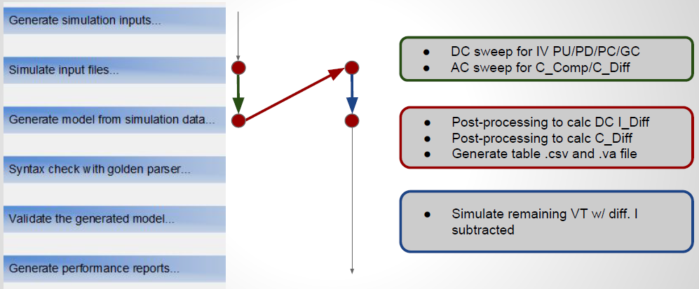
Modeling of the IV data:
While PU/PD is steady state DC sweep in theory, their simulation is performed in “pseudo DC” most of the time due to likely existence of clock signal, thus not possible for true DC sweep. In “pseudo-DC” simulation, voltage are swept very slowly. In addition, sweeping along X coordinate of different Y values are mutually independent. So they can be simulated in parallel (multi threaded or can be distributed). Simulation under certain biasing condition may have convergence issue, so a flow must be tolerant about missing sweep data on some grid points due to non-convergence.
In our SPIBPro example below, sweep of different Y bias points (e.g. voltage at output N) are separated in different .sp files and they can be simulated in parallel.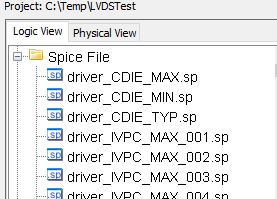
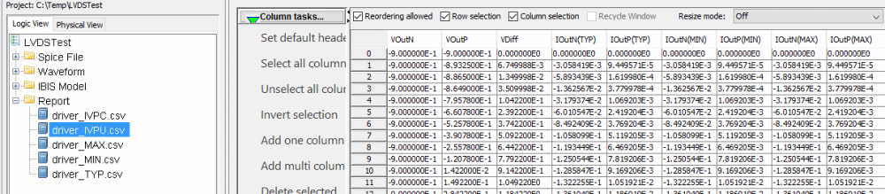
The task of post-processing step in the first iteration is to extract the simulation data just swept, calculate common-mode current, shift the surface data vertically, summarized as a table output and also perform initial modeling. Such a table is important for user to validate the the result and also perform some what-if modeling using tool like Excel if neded.
-
Surface modeling:
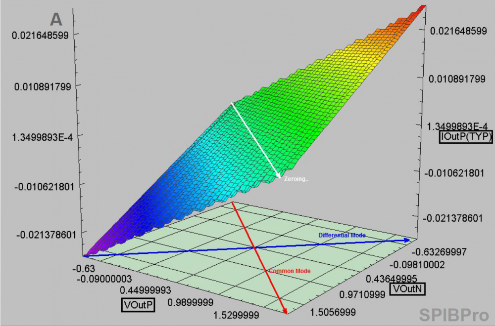
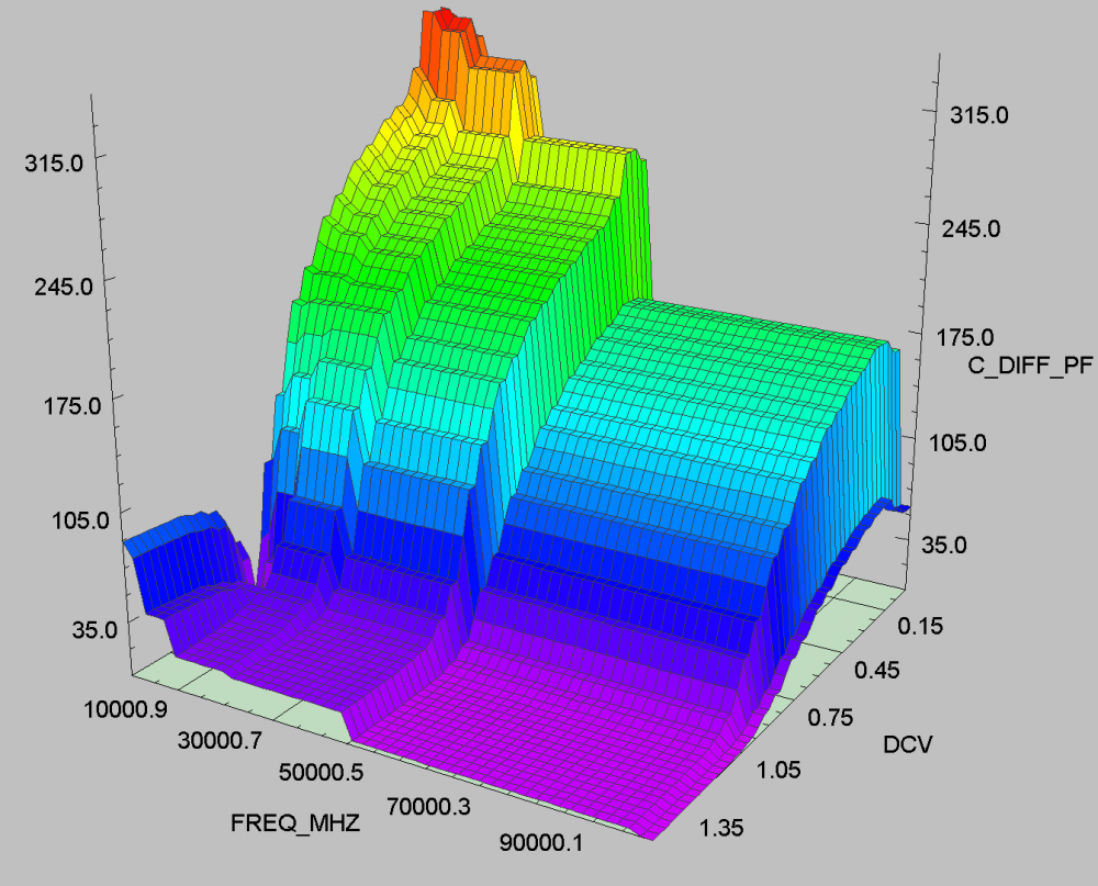
Depending on the symmetric differential mode data of shifted surface table (data on the surface alone the blue line), one may decide whether it’s pure resistive, linear or non-linear. The symmetric differential mode is orthogonal to the zeroed common mode curve (red straight line) and it represents the most likely differential operation (i.e. symmetric output of P and N) For example, the surface plot below suggest a resistor will suffice for the content of the series element:
With the csv table, one can quickly confirm whether the resistance is same across different voltage or not. If positive, then a linear resistor can be used. Otherwise, the non-linear resistance need to be modeled either with PWL spice element or as a series current (another IV table) in the series element. To be able to visualize the data with certain degrees of manipulation, a flow needs to have such 3D plotting capabilities. Otherwise, tool like matlab and familiarity of its syntax becomes necessary.
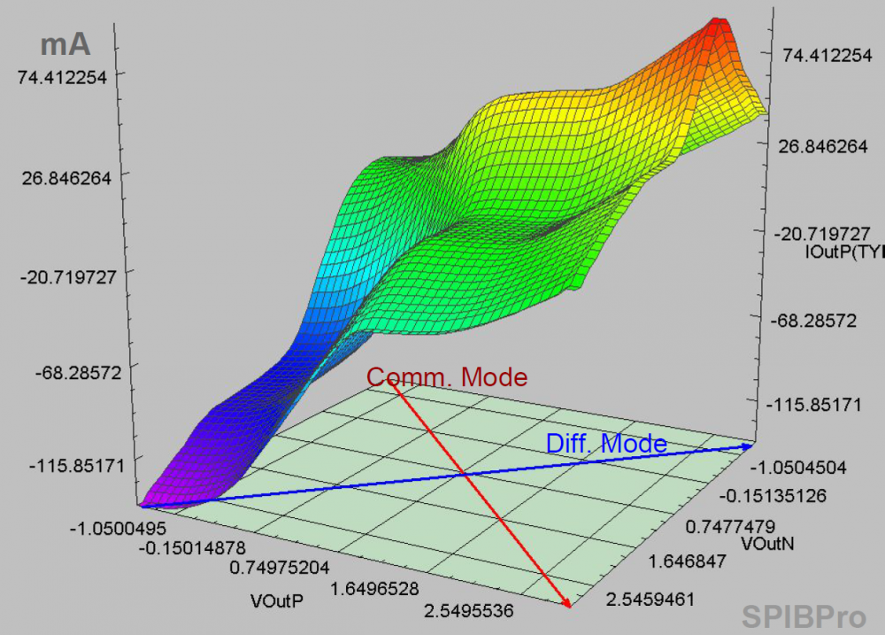
If the sweeping data shows surface like above, then either a surface modeling is needed or a “series MOSFET” needs to be created as a series element. For surface modeling, one can use “response surface modeling” like method to calculate fitting coefficients in minimizing the mean squared error sense. Other general modeling approach like neural network is certainly also possible.
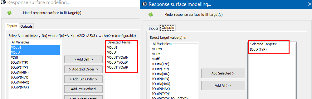
One should also check the residue of the prediction formula and maybe visualized as a scattered plot. SPIMPro’s general modeling and plotting functions are demonstrated below:
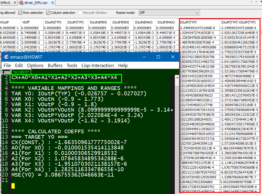
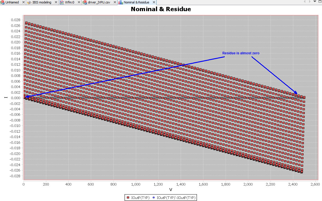
A good fit should have very small residue, shown as grey line across 0.0 in the picture above (other red dots are nominal values from sweeping grids). With valid results, one will need to translate this “prediction formula” into spice netlist using E/F/G/H control elements.
In matlab, similar process can be done using “lsfit” function.
- Series element:
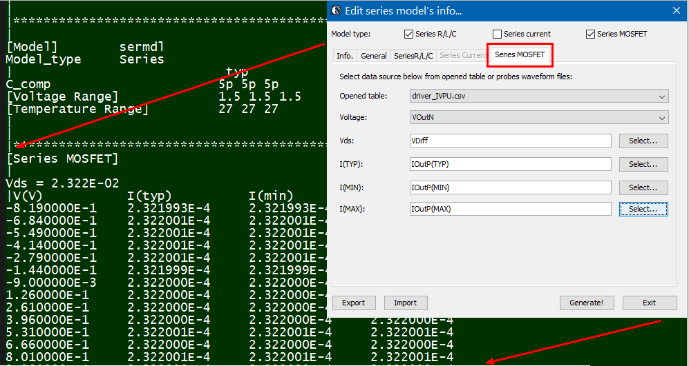 The same table content is sufficient to construct a series element. The steps needed here is to translate data into a IBIS compatible format. Such process is trivial when the model is simply R/L/C. For series current and series MOSFET (can have up to 100 tables of different bias condition), the attention needed to perform such work manually is not economical and a tool/flow should be used instead.
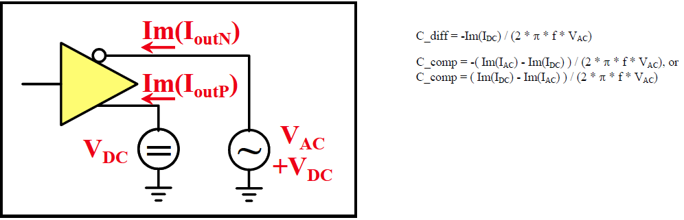
Modeling of the C-Diff:
Similar process (tabulated and modeling) can be applied to calculated C_Diff. However, it’s much more limited in terms of series element’s syntax and E/F/G/H equation such that describing such surface (both frequency and voltage dependent) for C_Diff is not practical using either spice or series element. As a result, a trade-off needs to be made when picking values (or to average) from the surface and a single value is used when constructing model for C_Diff.
Verilog-A modeling:
In our submission to the IBIS summit later this year, we proposed another flow which is Verilog/VHDL based. One of the advantages of this implementation is that the raw, table-like data can be used directly using built-in $table_model function. Its usage also enables polarity differentiation and elaborated description of C_Diff, which is very crucial to the transient data accuracy. The details about this will be published here once our paper is accepted.
Combined model:
In previous post, we mentioned that in addition to the “series element” for differential model, pure [External Model] of the differential model type may also be used. Using the proposed Verilog-A/VHDL for series element only model, these two methods can then work together, as shown below:
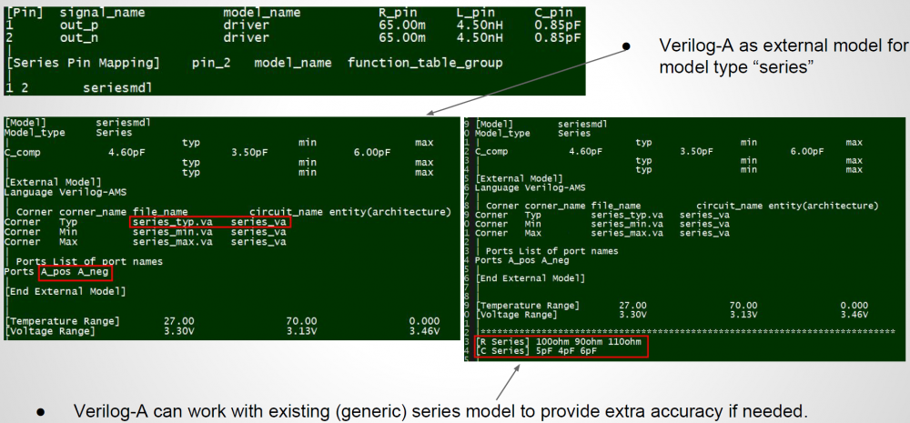
A series model is still declared in the “[Series PIn Mapping]” section to be connected between buffer’s N and P outputs. Its definition, can optionally include an external model such as the one implemented with behavioral language. This “[external model]” works on top of existing series model definitions and can provide extra info. such as frequency/voltage dependent C_Diff if the simulator supports. Optionally, the “top” series model can be simply a shell (e.g. with high impedance) and all the info. regarding the differential current is encapsulated inside the added model. When comparing to external model attached under output/IO buffer, this external model can be significantly less complicated and also provide more tuning capabilities.
Differential flow validation:
To validate a differential modeling flow, one may construct a differential buffer by creating an artificial coupling (e.g. using some R/C elements) and then connect it between two known IBIS buffers. During the validation, the calculated common-mode data from DC sweep should reconstruct exactly the same PU/PD/PC/GC tables as those in the known IBIS buffer. Differential current will reveal the resitive element of the coupling portion. Calculated C_Diff should reveal the coupling capacitive element. Both of these steady state differential current and C_Diff can be validated using generated csv table or raw data. User should then find that with both captured accurately, the transient VT data calculated will also correlate to those of original IBIS buffer very well.
Paper and audio recording:
We presented this study at the 2016 Asian IBIS Summits. Readers may download the presentation from IBIS website or [HERE]. Audio recording at Tokyo is also available [HERE]
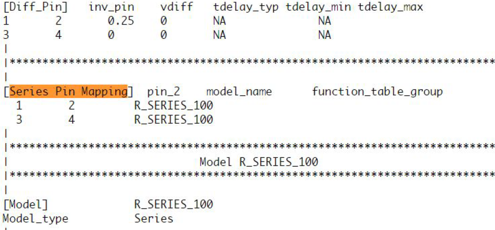 Take the picture shown above as an example. Under the “Series Pin Mapping” keyword, a model named “R_SERIES_100” is declared to connect pin 1 to and 2. Another instance of such model also sit between pin 3 and 4. Pin 1~4 each has its own model defined in other part of the ibis file already. For example, pin 1, 2 may have an output buffer connected while pin 3, 4 have open-drain buffers. This R_SERIES_100 model must have type “Series” defined as part of the IBIS file. Since “Series” is one of predefined IBIS model type, its contents (keywords) are not free form and must be one or more of the following series elements: R, L, C, Series current and Series MOSFET which contains up to 100 I/V tables under different biasing voltages.
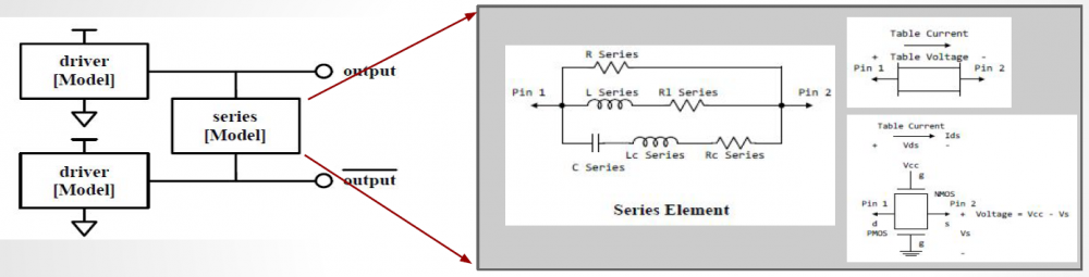
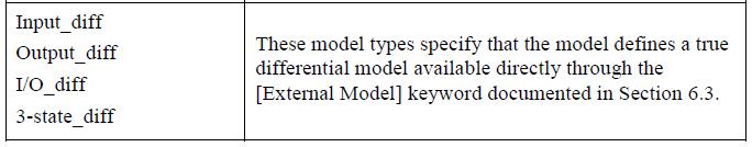 These differential model types must be implemented with language such as Spice, VHDL-AMS, Verlog-AMS, IBIS Interconnect Spice Sub-circuits (IBIS ISS) and declared with the “External” model section. These languages provides much more flexibility in terms of modeling capabilities, yet they also diminish the portability of the generated IBIS model.
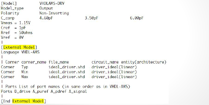 In the example above, a separate file “ideal_driver.vhd” must be provided outside the IBIS file and an “entity” of name “driver_ideal” needs to be defined. The port connections is described using reserved keywords after the “Ports” statement. In the IBIS Spec, all possible ports are pre-defined and the declaring order here must match their definitions in the associated Verilog/VHDL etc file.