[This blog post is written in preparation for the presentation of the same title to be given at the 2018 DesignCon IBIS Summit. Presentation slides and audio recording are linked at the bottom of this post.]
Motivation:
An AMI model is in the binary form of .dll (dynamic link library) or .so (shared object). It itself is not an executable and can’t be used directly. To load or run the AMI models, one needs to have a “driver”. Commercial tools like HSpice has a license required utility called “AMICheck” to test drive the given AMI models with rise/fall/single bit response. We SPISim also provide a free utility called SPISimAMI.exe which does pretty much the same. These small drivers are good when you want to quickly check whether the AMI models at hand are “run-able”. However, to validate or test model’s full function, such a simple tester is often insufficient. In an ideal situation, a link analysis simulator, which will load Tx and Rx AMI models involved and perform calculation/optimization, is preferred as a driver. If a model developer can use IDE to attach to this simulator process and have access to the simulator codes as well, then he/she can set a break point within both simulator and the loaded AMI model to step through and debug during the whole analysis process.
Even if one doesn’t have access to simulator’s codes or debug build, theoretically, an IDE can also “attach” to a process before it loads the AMI dlls in which we have break points set (as a model builder, we have access to the model codes). However, thing is not so straight forward in real world. Most of the EDA tools I have seen allow user to interact different link analysis settings via GUI, then when a “simulate” button is clicked, a separated process is launched/forked and that process will do the work such as characterizing channel, loading AMI models and simulation etc before giving results back to the front-end GUI for further display. It is not easy (if even possible) to automatically attach dll files being debugged to these “spawn/forked” process. No to mention that if both Tx and Rx models are involved in a optimization process (such as back-channel), then simply stopping at a breaking point within one of the AMI models is not enough… one can’t observe and see the interactions for full picture. With these limitations, develop and testing AMI models within a full link analysis flow become challenging.
For a model developer who does not have access to these full link simulator’s sources, open source platform is a direction. There are several ones out there already… PyBert and COM are two such examples. From what I have seen, most of them already have some generic Tx/Rx algorithm blocks in place. So these EQ operating portions may be replaced to support AMI models to meet our needs. Being able to do so will shorten the model design cycle and enable the possibility to develop blocks with more advanced capabilities (such as back-channel communication). As PyBert already has some sort of AMI modeling support, this paper intends to explore possibilities to add similar capabilities in IEEE 802.3 spec. supported channel operating margin (COM) flow.
Background:
Channel Operating Margin (COM) is a ratified IEEE802.3 spec. Interested reader can find an overview slides given by the COM main author (also my former colleague at Intel) linked here: [Channel Operating Margin Tutorial] More detailed technical details are available in the IEEE 802.3BJ spec document and Richard’s 2013 DesignCon paper of same title. Further more, its matlab source codes are also available at the 802.3 website.
Given such technical depth like COM’s, to describe it in several paragraphs in this post will not be meaningful. So I will try to just give an overview from AMI builder’s perspective and help reader to see how AMI models can be plugged-in to the flow.
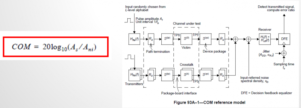
COM’s reference model is shown above. The upper half of the right side represent the through inter-symbol-interference (ISI) channel and the lower half is for the crosstalk (XTK), which can be near end, far end or both. Simply put, COM is an evaluation of signal to noise ratio for the full system. Most of the noise terms, such as mentioned ISI, XTK, jitters etc have all been taken into account. The signal part is the peak of the single bit response (SBR, i.e. pulse response). COM itself has published algorithms for many different blocks above and also interface specific default parameters for different 803.2 interfaces. EQ portion such as FFE in Tx, CTLE in Rx and even DFE are also implemented.
For a SERDES designer or AMI model builder, channel S-param (with or without package portion) is assumed given and COM flow will select best selection of FFE tap weights, CTLE pole/zero location and DFE tap weights as well. The searching flow for these parameters are exhaustive… full combination of FFE taps and CTLE dc gains are used to apply for toward the channel. A figure of merit (FOM) is then calculated for each combination. Best case is then decided based on the FOM value. Once EQ settings have been decided, then a SBR is formed and a full blown BER like analysis is applied with DFE involved to calculate final COM value.
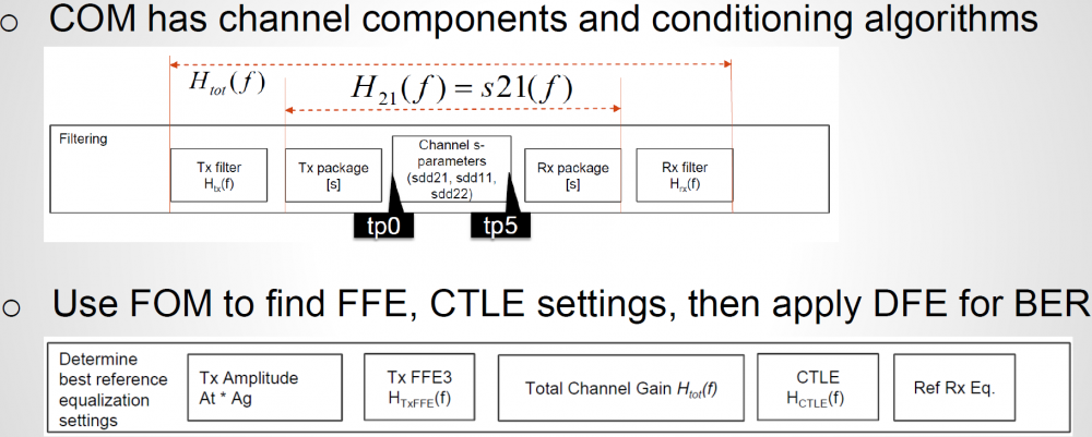
For a link analysis flow, the first step is to “characterize” the channel, i.e. obtain impulse response. There are many devil’s details behind this step… single-ended s-param may be need to converted to mixed mode, package models of different sections needs to be cascaded, and finally the cascaded s-param needs to be “conditioned” before doing IFFT (not using an IBIS model or analog front-end in COM). All of these are important yet may be out of an AMI model builder’s direct concern… then just want this channel to “work”. Fortunately, these steps have all been included in COM flow already and can be used as they are.
Regarding Tx and Rx EQ, original COM implementation (circa. 2014) only supports one FFE pre-tap and one post-tap for TX. Recently, it have been extended to support two pre-tap and three post-taps. For CTLE, two poles and one zero equation is used and user can only sweep DC gain. The analysis flow is very similar to what’s described in IBIS spec section 10.2 but only with LTI assumption. That is, impulse response obtained from conditioned S-param is sent to Tx EQ, then pass through Rx CTLE before further processing. DFE taps are not optimized within each iteration of FOM calculation, it’s calculated only after optimized FFE + CTLE settings have been found.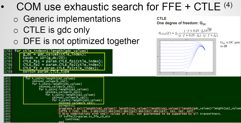
As mentioned previously, the searching algorithm of these EQ is exhaustive. So if one open the published COM matlab codes, he/she will find the multi-level loops for different Tx EQ taps and Rx CTLE Gdc settings as shown above. To replace these generic EQ functions with our AMI models, codes need to be changed here.
Using AMI in COM flow:
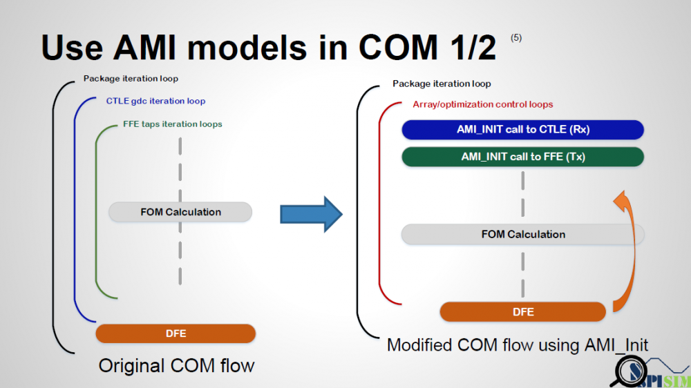
To use AMI model in a COM flow, one need to replace collect the replace these FFE and CTLE calls in the COM codes with the corresponding AMI model invocation. Here shows two possible modifications routes:
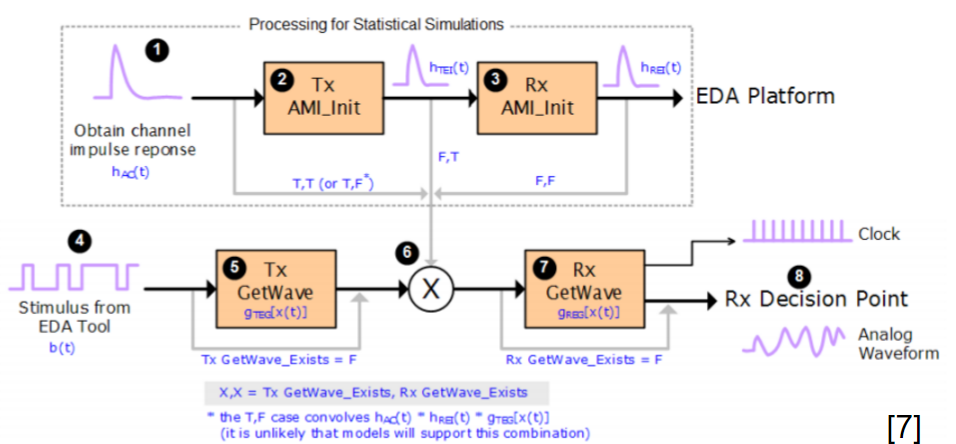
- LTI (Linear, time invariant) design: As COM flow use impulse response by default, it’s easier to plug-in LTI AMI model (i.e. models which don’t use AMI_GetWave to process data) directly.
The first step is to “combine” or “collapse” those multi-level loops into single loop. This single loop can be iteration which go through an array which contains all the AMI parameters combinations to be tried (may not be exhaustive) or has a “stopping-criteria” which will “break” the loop such as optimization within this single loop has reached solution. Tx and Rx may not be FFE/CTLE respectively or can have different format (for example, CTLE can iteration list of frequency response curves rather than pole/zero data). For the later case (optimization), Tx and RX can be calculated together if needed. original COM’s package length and DFE can still be used to calculate FOM of different condition if needed.
- NLTV (Non-linear, Time variant) design: In this case, a PRBS like bit-pattern is needed first in order to convolve with the channel’s impulse response. Bit-stream response is then formed to feed into model’s AMI_GetWave function within each loop. Just like what’s described in IBIS’s spec, Tx and Rx’s GetWave functions are called sequentially and model’s DFE and FOM function (not COM’s) may be used at the end to decide when to finish the iteration.
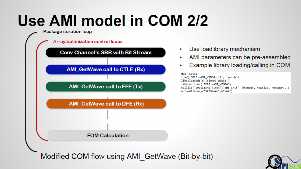
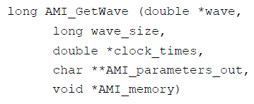
Regarding implementation details, as COM was originally written in matlab, so matlab’s corresponding mechanism to load and call external DLL functions need to be used to replace original FFE/CTLE function call. Basically (as shown in the right part of the picture above), mex -setup needs to be called to determine which IDE environment is installed in the working computer. A header file which include the definitions of the AMI API function is also needed. Then the following functions are called in sequence:
- Load AMI model using: load(‘XXXXXX.dll’, ‘ami.h’)
- check libisloaded(‘XXXXXX’) and list functions in the library using libfunctions(XXXXXX’)
- Call AMI library function using calllib(‘XXXXXX.dll’, ‘ami_init’, htInput, rowSize…)
- Finally unloadlibrary(‘XXXXXX’)
Also worth mentioned is that if we are doing this for AMI models being developed, not a generalized AMI-capable link simulator, then parser for .ami to form parameter tree is not necessarily needed to form argument passing into ami_init functions etc. We can form a string of parsed “key-value” pairs in advance manually and pass into AMI function. Other open platform like PyBert does have AMI parser built-in for its AMI capabilities.
Results:
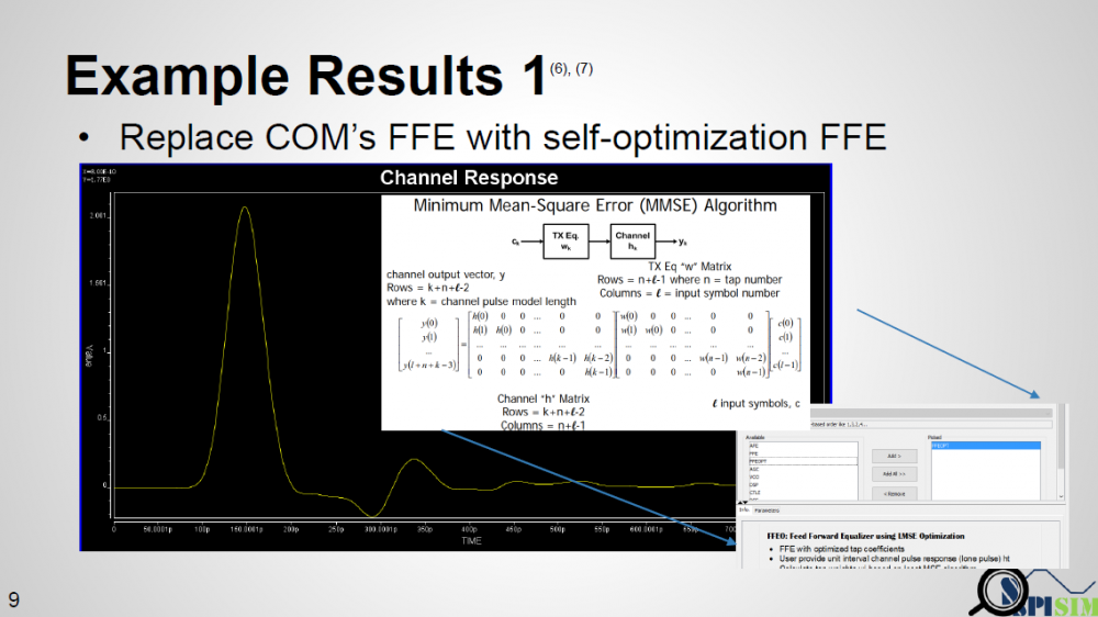
In our experiment, we want to avoid the multi-level loops for all possible FFE tap weight combinations by using our AMI FFE model capable of self-optimization. The concept is simple: if we already have an channel’s impulse response, then the optimal weight to obtain same output as input (recover signal) in the minimum mean-squared error sense can be solved by using pseudo-inverse and linear algebra technique. We want to validate this approach work and can find similar (if not same) solution comparing to full exhaustive search.
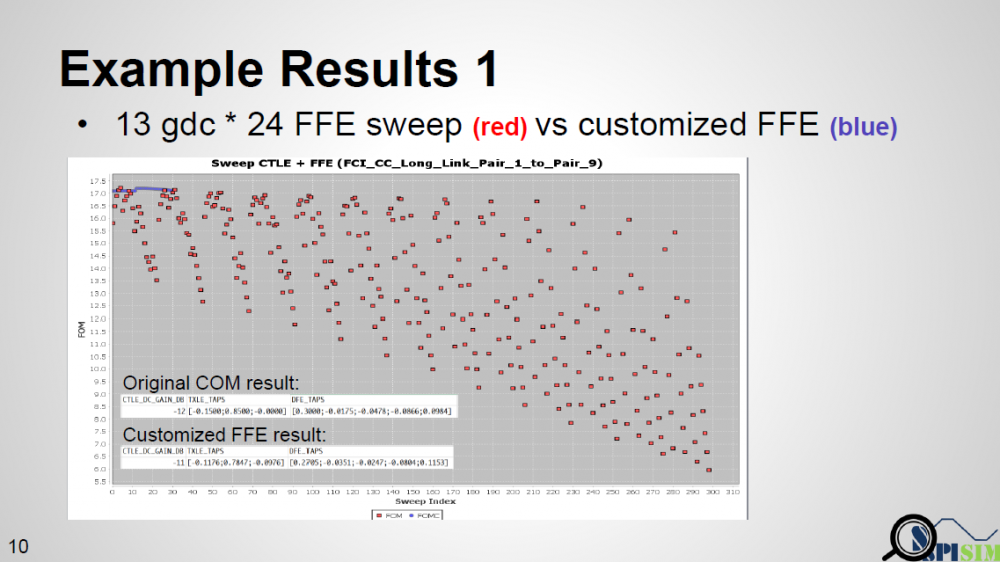
Result is shown above. Red dot represents original COM’s sweeping results (FOM value). There are 13 Gdc values each with 24 one pre-tap and one-post tap combination possible… so total 312 run is needed. Blue dots are our AMI results… since we still use COM’s CTLE, so 13 run is performed. However, for each Gdc run, AMI model computes only once based on the self-optimization algorithm mentioned and finally report best results together with best CTLE Gdc. As seen that blue dots are almost at the top of all 13 original ” COM chunks”, we validate that this algorithm/our Optimization-capable FFE does work.
Summary:
To summarize this study, first we want to emphasize that for a model developer, who can be an individual model provider or a SERDES designer being asked to develop AMI models, a full flow capable of being used to debug AMI model being developed is needed. This can’t be covered by the simple utility driver particular when optimization such as back-channel come into play.
To meet our needs, open-source link-analysis platform is worth considering. In particular, COM flow of IEEE802.3 is attractive because it’s been ratified, well documented, widely used and support BER-like flow with source codes. While its Tx and Rx block functions may be generic, it’s not difficult to replace those function calls with our own AMI models’ API functions in either LTI or NLTV scenarios. This process not only help shortening model development cycles, but also is very beneficial in further understanding how link analysis is actually performed.
Links:
Presentation: [HERE] (http://www.spisim.com/support/paperetc/20180202_DesignConSummit_SPISim.pdf)
Audio recording (English): [HERE]