

Overview:
Continuous time linear equalizer, or CTLE for short, is a commonly used in modern communication channel. In a system where lossy channels are present, a CTLE can often recover signal quality for receiver or down stream continuous signaling. There have been many articles online discussing how a CTLE works theoretically. More thorough technical details are certainly also available in college/graduate level communication/IC design text book. In this blog post, I would like to focus more on its IBIS-AMI modeling aspect from a practical point of view. While not all secret sauce will be revealed here:-), hopefully the points mentioned here will give reader a good staring point in implementing or determining their CTLE/AMI modeling methodologies.
[Credit:] Some of the pictures used in this post are from Professor Sam Palermo’s course webpage linked below. He was also my colleague at Intel previously. (not knowing each other though..)
ECEN 720: High-Speed Links Circuits and Systems
What and why CTLE:
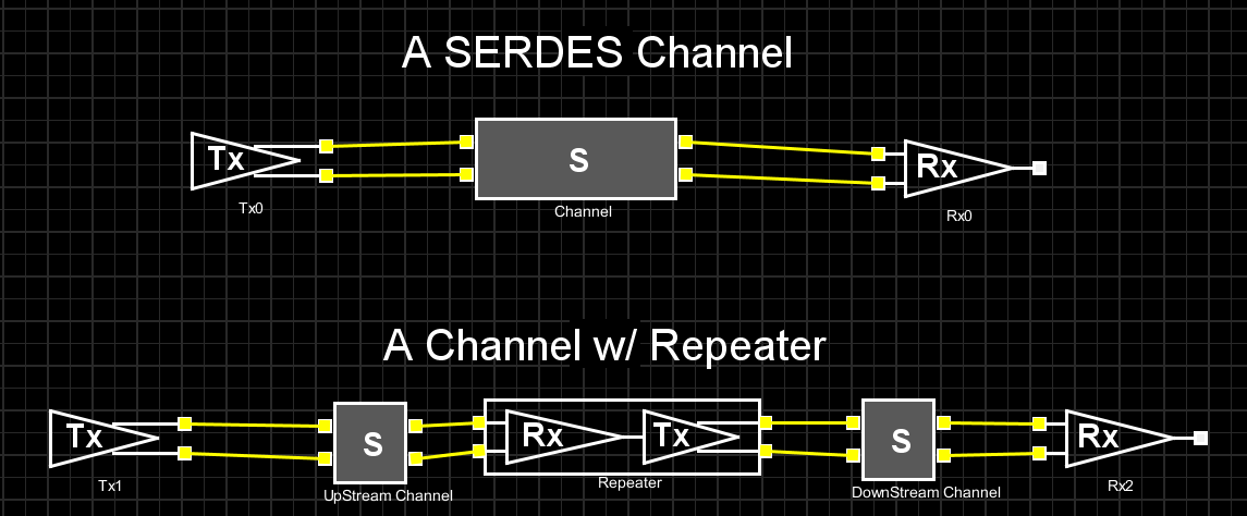
The picture above shows two common SERDES channel setups. While the one at the top has a direct connection between Tx and Rx, the bottom one has a “repeater” to cascade up stream and down stream channels together. This “cascading” can be repeated more than once so there maybe more than two channels involved. CTLE may sit inside the Rx of both set-ups or the middle “ReDriver” in the bottom one. In either case, the S-parameter block represents a generalized channel. It may contain passive elements such as package, transmission lines, vias or connectors etc. A characteristic of such channel is that it presents different losses across spectrum, i.e. dispersion.
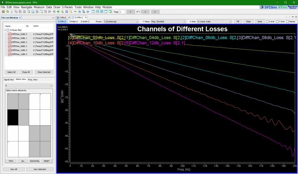
For example, if we plot these channel’s differential input to differential output, we may see their frequency domain (FD) loss as shown above.
Digital signals being transmitted are more or less like sequence of bit/square pulse. We know that very rich frequency components are generated during its sharp rising/falling transition edges. Ideally, a communication channel to propagate these signals should behave like an (unit-gain) all pass filter. That is, various frequency components of the signal should not be treated equally, otherwise distortion will occur. Such ideal response can be indicated as the green box below:
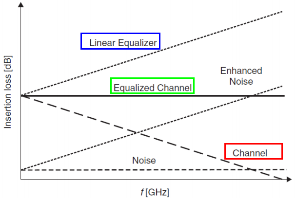
In reality, such all pass filter does come often. In order to compensate our lossy channels (as indicated by the red box) to be more like the ideal case (green box) as an end result, we need to apply equalization (indicated by blue box). This is why an equalizer is often used… basically it provides a transfer function/frequency response to compensate the lossy channel in order to recover the signal quality. A point worth taken here is that the blue box and red box are “tie” together. So using same equalizer for channels of different losses may cause under or over compensated. That is, an equalizer is related to the channel being compensated. Another point is that CTLE is just a subset of such linear equalizer.
CTLE is a subset of linear equalizer:
A linear equalizer can be implemented in many different ways. For example, a feed-forward equalizer is often used in the Tx side and within DFE:
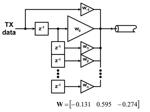
FFE’s behavior is more or less easier to predict and its AMI implementation is also quite straight forward. For example, a single pre-tap or post-tap’s FFE response can be easily visualized and predicted: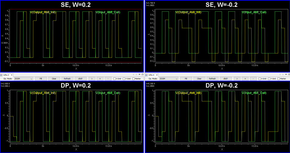
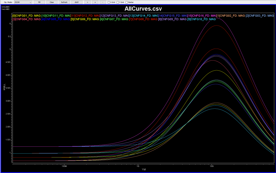
Now, a CTLE is a more “generalized” linear equalizer, so its behavior is usually represented in terms of frequency responses. Thus, to accommodate/compensate channels of different losses, we will have different FD responses for CTLE:
Now that IBIS-AMI modeling for CTLE is of concern, how do we obtain such modeling data for CTLE and how they should be modeled?
Different types of CTLE modeling data:
While CTLE’s behavior can be easily understood in frequency domain, for IBIS-AMI or channel analysis, it eventually needs to come back to time domain (FD) to convolve with inputs. This is because both statistical or bit-by-bit mode of link analysis are in time domain. Thus we have several choice: provide model FD data and have it converted to TD inside the implemented AMI model, or simply provide TD response directly to the model. The benefit of the first approach is that model can perform iFFT based on analysis’ bit rate and sampling rate’s settings. The advantage of the latter one is that the provided TD model can be checked to have good quality and model does not need to do similar iFFT every time simulation starts. Of course, the best implementation, i.e. like us SPISim’s approach, is to support both modes for best flexibility and expandability 🙂
- Frequency domain data:
Depending on the availability of original EQ design, there are several possibilities for FD data: Synthesized with poles and zeros, extract from S-parameters or AC simulation to extract response.
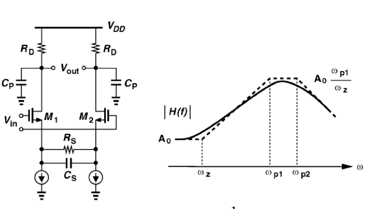
- Poles and Zeros: Given different number of poles, zeros and their locations along with dc boost level, one can synthesize FD response curves:
 So say if we are given a data sheet which has EQ level of some key frequencies like below:
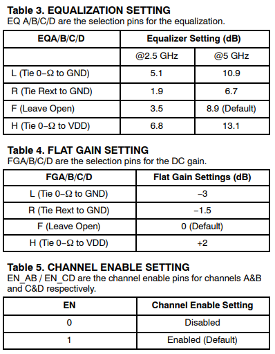 Then one can sweep different number and locations of poles and zeros to obtain matching curves to meet the spec.:
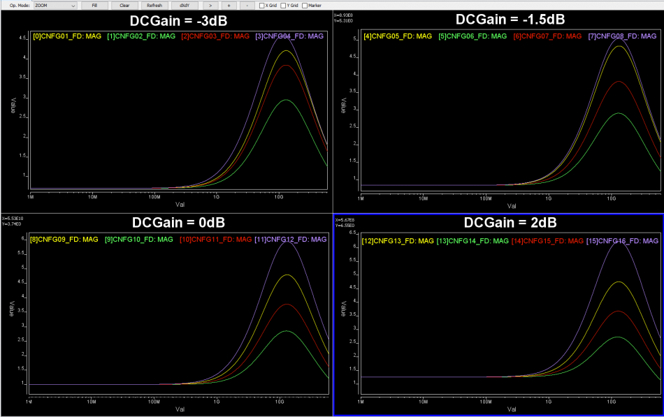 Such synthesized curves are well behaved in terms of passivity and causality etc, and can be extended to covered desired frequency bandwidth.
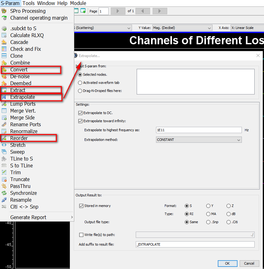
 - Extract from S-parameters: Another way to obtain frequency response is from EQ circuit’s existing S-parameter. This will provide best correlation scenarios for generated AMI model because the raw data can serve as a design target. However, there are many intermediate steps one have to perform first. For example, the given s-parameter may be single ended and only with limited frequency range (due to limitation of VNA being used), so if tool like our SPISim’s SPro is used, then one needs to: reording port (from Even-Odd ordering, i.e. 1-3, 2-4 etc to Sequential ordering, i.e. 1, 2 -> 3, 4), then convert to differential/mixed mode, after that extrapolate toward dc and high frequencies (many algorithms can be used and such extrapolation must also abide by physics) and finally extract the only related differential input -> differential output portion data.
- AC simulation: This assumes original design is available for AC simulation. Such raw data still needs to be sanity checked in terms of loss and phase change. For example, if gain are not flat toward DC and high-frequency range, then extra fixing may be needed otherwise iFFT results will be spurious.
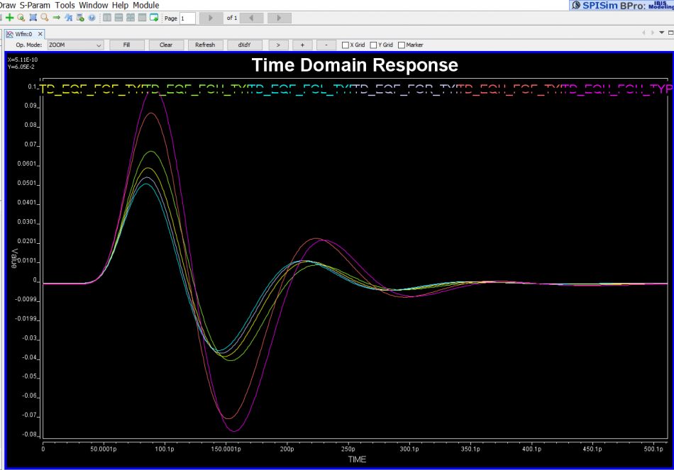
- Time domain data: time domain response can be obtained from aforementioned FD data by doing iFFT directly as shown below. It may also be obtained by simulating original EQ circuit in time domain. However, there are still several considerations:
- How to do iFFT: padding with zeros or conjugate are usually needed for real data iFFT. If the original FD data is not “clean” in terms of causality, passivity or asymptotic behavior, then they need to be fixed first.
- TD simulation: Is simulating impulse response possible? If not, maybe a step response should be performed instead. Then what is the time step or ramp speed to excite input stimuli? Note that during IBIS-AMI’s link analysis, the time step being used there may be different from the one being used here, so how will you scale the data accordingly. Once a step response is available, successive differentiation will produce impulse response with proper scaling.
How to implement CTLE AMI model:
Now that we have data to model, how will they be implemented in C/C++ codes to support AMI API for link analysis is another level of consideration.
- Decision mechanism: As mentioned previously, a CTLE FD response targets at a channel of certain loss, thus the decision to use appropriate CTLE settings based on that particular channel at hand must either be decided by user or the model itself. While the former (user decision) does not need further explanation, the latter case (model decision, i.e. being adaptive) is a whole different topic and often vendor specific.
Typically, such adaptive mechanism has a pre-sorted CTLE in terms of strength or EQ level, then a figure-of-merit (FOM) needs to be extracted from equalized signal. That is, apply a tentative CTLE to the received data, then calculate such FOM. Then increase or decrease the EQ level by using adjacent CTLE curves and see whether FOM improves. Continue doing so until either selected CTLE “ID” settles or reach the range bounds. This process may be performed across many different cycles until it “stabilized” or being “locked”. Thus, the model may need to go through training period first to determine best CTLE being used during subsequent link analysis.
- EQ configurations:
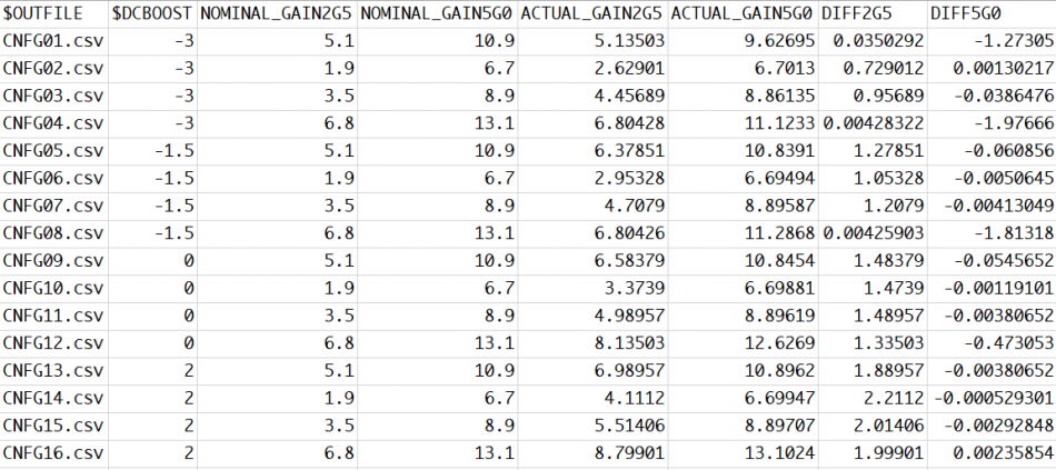
So now you have a bunch of settings or data like below, how should you architecture the model properly such that it can be extended in the future with revised CTLE response or allow user to perform corner selections (which essentially adds another dimension):
This is now more in software architecture domain and needs some trade-off considerations. For example, you may want to provide fine grid full spectrum FD/TD response but the data will may become to big. So internal re-sampling may be needed. For FD data, the model may needs to sample to have 2^N points for efficient iFFT. Different corner/parameter selection should not be hard coded in the models because future revised model’s parameter may be different. For external source data, encryption is usually needed to protect the modeling IP. With proper planning, one may reuse same CLTE module in many different design without customization on a case-by-case basis.
- Correlations:
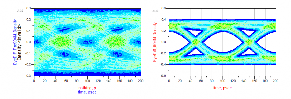
Finally it’s time to correlate the create CTLE AMI model against original EQ design or its behavioral model. Done properly, you should see signals being “recovered” from left to right below:
However, getting results like this in the first try may be a wishful thinking. In particular, the IBIS-AMI model does not work alone… it needs to work together with associated IBIS model (analog front-end) in most link simulator. So that IBIS model’s parasitics and loading etc will all affect the result. Besides, the high-impedance assumption of the AMI model also means proper termination matching is needed before one can drop them in for direct replacement of existing EQ circuit or behavioral models for correlation.
Summary:
At this point, you may realize that while a CTLE can be easily understood from its theoretic behavior perspective, its implementation to meet IBIS-AMI demands is a different story. We have seen CTLE models made by other vendor not expandable at all such that the client need to scratch the existing ones for minor revised CTLE behavior/settings (also because this particular model maker charges too much, of course). It’s our hope that the learning experience mentioned in this post will provide some guidance or considerations regardless when you decide to deep dive developing your own CTLE IBIS-AMI model, or maybe just delegate such tasks to professional model makers like us 🙂