In system analysis, signal integrity is done in either pre-layout and post-layout phase. Power integrity (PI), on the other hand, deals with mostly post-layout data. Layout is usually generated manually and then simulated in time consuming 3D solving process. As a result, optimization flow for PI is quite different from that for SI and is also very problem specific.
Power Integrity:
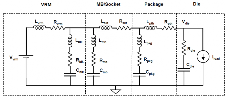
Power delivery model
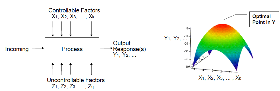
Power integrity aims at providing “clean” voltage supply to active elements in the channel such as driver and receiver. A typical representation of power delivery network is shown above, it starts with the voltage regulation and includes the motherboard, the package, and the die itself. Due to the impedance associated with the power delivery loop, any current through this loop will cause a drop in the voltage available to the die. Current is supplied from voltage regulator ultimately but is also stored in the de-coupling capacitors on the conducting path.This drawing current (Icct or Iload) varies due to different number of buffers switching at different frequency or work load… This drop in the voltage at the die directly impacts the maximum operating frequency of the design. Thus a spec. must be provided and met for the droop voltage to assure design quality.
The impedance in the power delivery loop can be classified as both resistive and inductive. The resistive drop is proportional to the current through the loop while the inductive drop is proportional to the rate of change of current. It is desired to have small loop inductance as Ldi/dt will contribute to the droop. This inductive drop is typically countered by adding several stages of decoupling caps at various points in the power delivery network. This helps reduce the overall impedance of the power delivery loop over a broad frequency range.
The conducting paths are layout design, rather than spice-like electrical netlist. The decoupling caps are usually provided by external vendors (e.g. Murata) and the designer needs to decide where and how to place them. So a power integrity analysis usually includes the following aspects:
- stackup, power via arrangement and pin out;
- decoupling strategy, choice of location, number and value of caps
Optimization w/ Design synthesis:
The power delivery network is layout design solved with 3D field solver. If designs can be generated via rule-based synthesis, then the design cycle can be shortened and many designs can be generated in advance. A batch-mode like process is then used to solve for different PDN models for comparison and trade-off study.
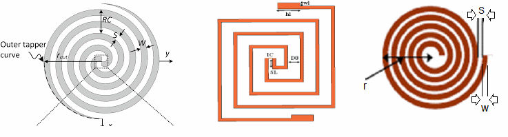
Take the different on-chip antennas shown above as an example, they are specified with different geometry parameters so that software algorithms is used to synthesize the design quickly. Do so manually may not be accurate or efficient. For a PD design, the rules are much more complicated than just the geometrical based parameters. Nevertheless, best practice or experienced based rules can still be summarized so that algorithm can perform the following tasks automcatically:
- Modify layer stackup thickness and material properties
- Generate pin, nodes, traces and shapes on specific layer either based on net name or reference location to other (signal or power) pins
- Generate (power) vias in certain pattern and connect to power/ground planes. Voids and proper pad-stacks are also generated as part of the process
- Duplicate certain region of the design (template) to other area as a X-Y array
- Perform DRC alone the way and generate warnings
The flow mentioned above is purposely built for a certain solver, it’s because different solver has its own definitions for different design object (via, traces, nodes etc) and the layout syntax is also solver specific. Nevertheless, this flow has great potential of shorten design cycle, permit design optimization via quick analysis of different design, and even reduce the needs for engineering layout resources.
Decoupling analysis:
Once decoupling strategy (land side caps and/or die-side caps) and corresponding layout is generated, a S-parameter for the PDN can be obtained via 3D field solving. With proper provision (not stuffing cap in advance in the design), this generated S-parameter may be used directly again and again for what-if decoupling analysis. If there is no layout/stackup change, 3D solving does not need to be repeated.
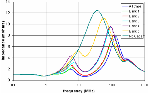
As shown above, different combination of caps “stuffed” at the output ports will cause impedance seeing into the die ports to vary. Conceptually, one may simulate the given S-parameter with cap connected and measure the impedance using simulation in frequency domain. In practice, such simulation is not needed as S-parameter can be converted into Y/Z-parameters and lumped together with cap’s FD impedance and be analyzed directly. As a result, we can post-process the PDN’s S-parameter for a certain decoupling cap arrangement to gain the following insights very quickly:
- The impedance (both inductive and resistive) of the PDN
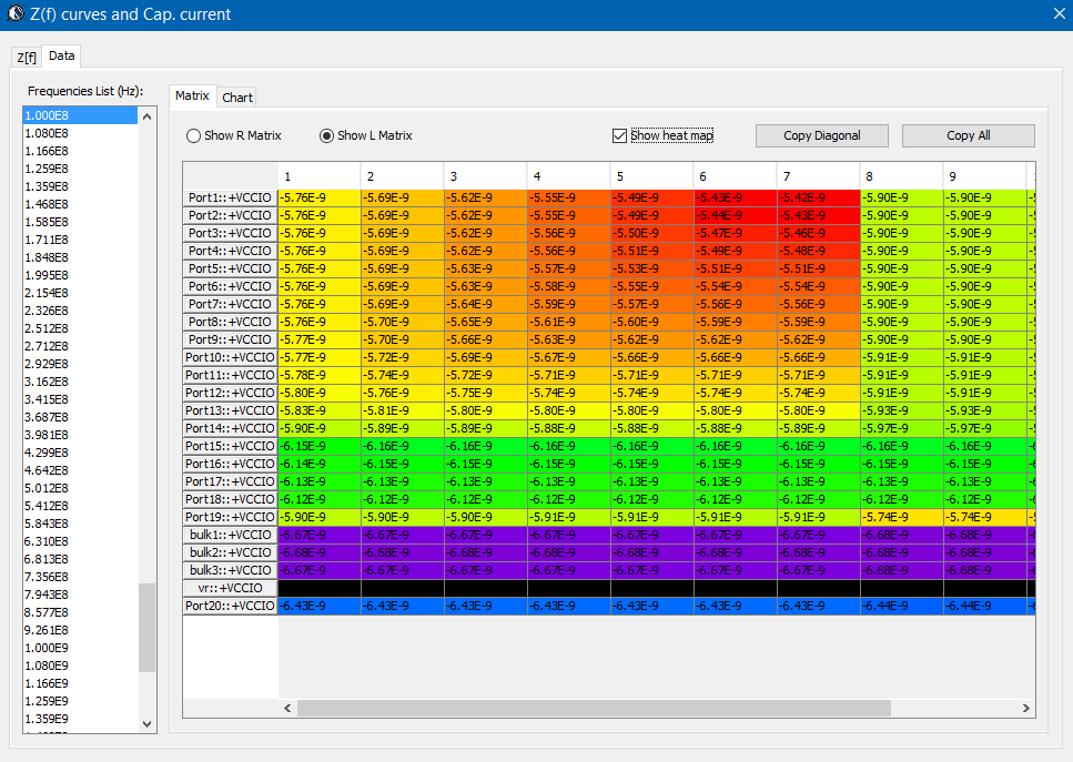
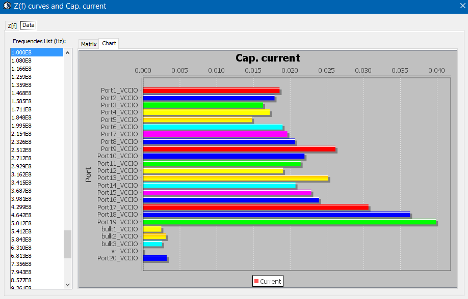
- Current contributed by each de-caps at certain frequency
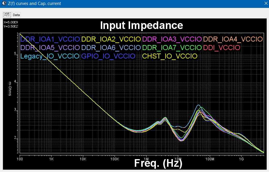
- Input impedance seen at each die-port
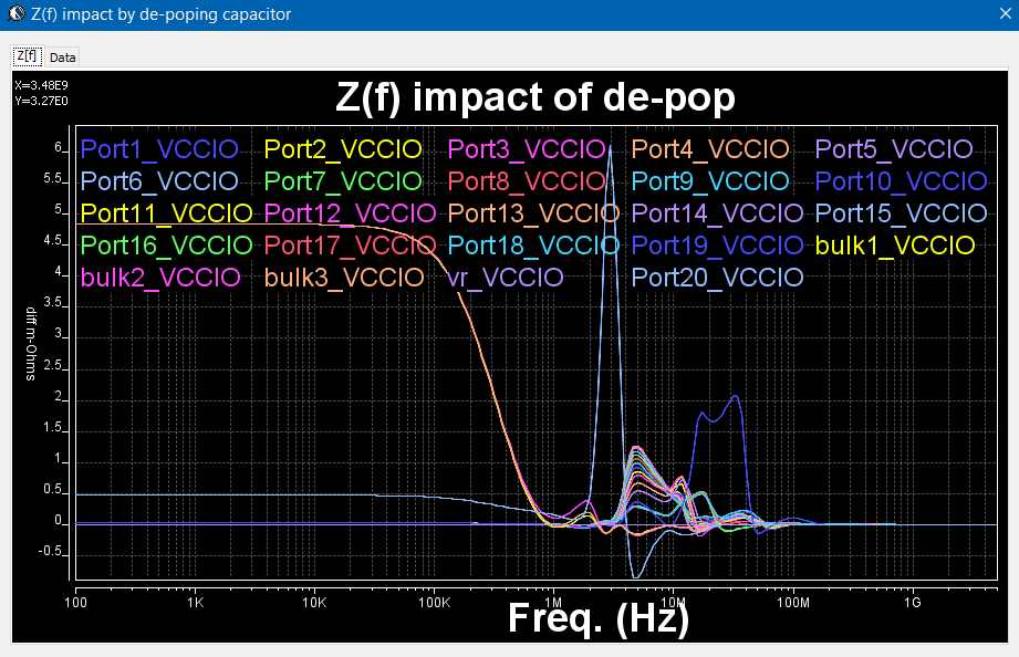
- Effective analysis: by removing a particular de-cap, how much impact does it have to the die’s impedance.
- How does this compare to different configuration: repeat the same “what-if” analysis for different configuration.

 Sources of noise affecting performance: