

IBIS-AMI modeling is a task usually executed at the end of IP development process. That is, hardward IPs are created first, then associated AMI models are developed and released to be accompany with this hardware IP since the IPs vendor usually does not want to expose the design details to the their customers. On the other hand, it is also likely the case that a user may have received behavioral or encrypted spice models first, or even obtain measurement data from the lab, then would like to create corresponding AMI models for channel analysis. Such needs arise usually because either original IP vendor does not have AMI model or may charge too much. It is also possible that end user would like to explore different design parameters before determining which IP/part to use.
In this post, we would like to discuss how such an usage demands can be accomplished with SPISim’s AMI flow without any C/C++ coding or compilation for AMI. Here are the topics for this case study:
- Collateral
- Design spec. and modeling goals
- Modeling process
- Model release
- Other thoughts
Collateral:
For this design, we received a testbench for a typical SERDES channel using this IP. The schematic is shown below: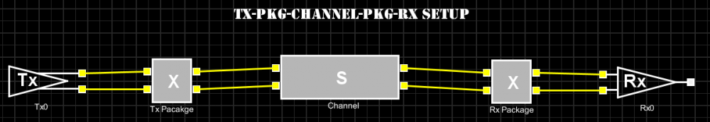
Both Tx and Rx are encrypted hspice models with adjustable parameters. When picking one set of parameters to test run the channel test bench, we get valid simulation results.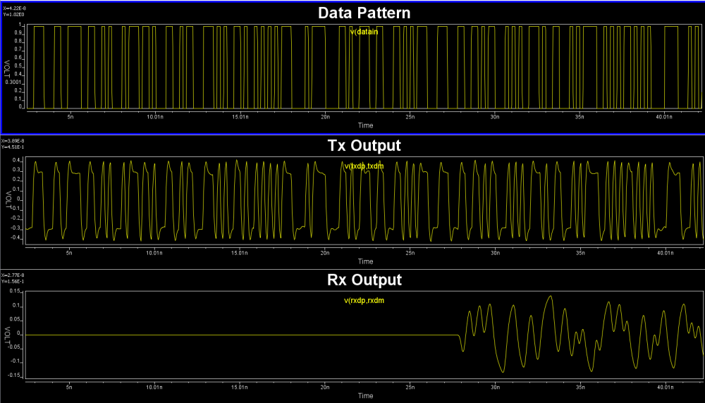
As this is a hspice netlist, we have the freedom to probe different points and change the simulation options as needed (for example, from transient to ac or transfer-function).
Design Spec. and modeling goals:
The original IP vendor only provides simple descriptions for various blocks and design parameters. The Tx and Rx packages are spice sub-circuits and channel is a s-parameter file. Both Tx and Rx model has typ/min/max corners. On the Tx side, there are settings for voltage supply which is independent with the corner settings, a 7-bit resolutions for a multiplier to work with the swing amplitude, a 6-bit resolution for a de-emphasis and a flag for turning-on/off the boost.
With these IP design spec, the modeling goal is to create associate AMI models which will allow end users to fine tune performance with similar parameters like original IP. Further more, SPIPro is used for its spec. AMI model so that model developer should not need to write any C/C++ codes or perform any .dll/.so compilation for this AMI modeling.
Modeling process:
If one needs to create AMI models from simulation or measurement results, that usually means he/she does not have original design details or even design spec. available. So the so called “top-down” approach will not work simply because there is no design at all to translate to corresponding C/C++ code. Instead, we need to create an architecture via trial-and-error to “reverse engineer” the design so that the performance will match what’s given. Here are the steps we used in this case:
- Create Tx/Rx test bench:
While the full channel test bench demonstrate how the Tx/Rx work, it also includes information not needed in the AMI modeling. For example, package and channel are usually separated from the AMI model because they are usage or client specific. Besides, as mentioned in previous posts, one assumption of AMI model is high-Z input and output. So the first step of the modeling is to separate channel from driver/receiver and create Tx and Rx only test bench together with inputs and outputs.
For Tx, it’s a simple PRBS input with output connecting to 50 ohms loads.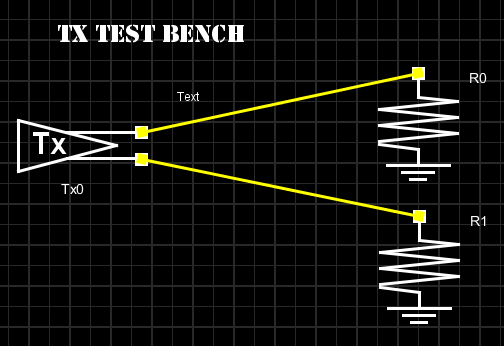
And its input/output should look like this:
When we modify the test bench to connect Tx directly to Rx, i.e. bypass all the package and channel models, we get such input/output eyes:
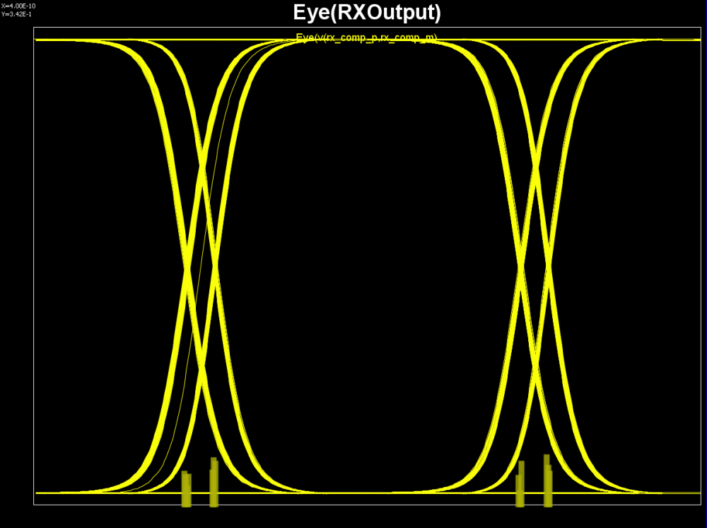
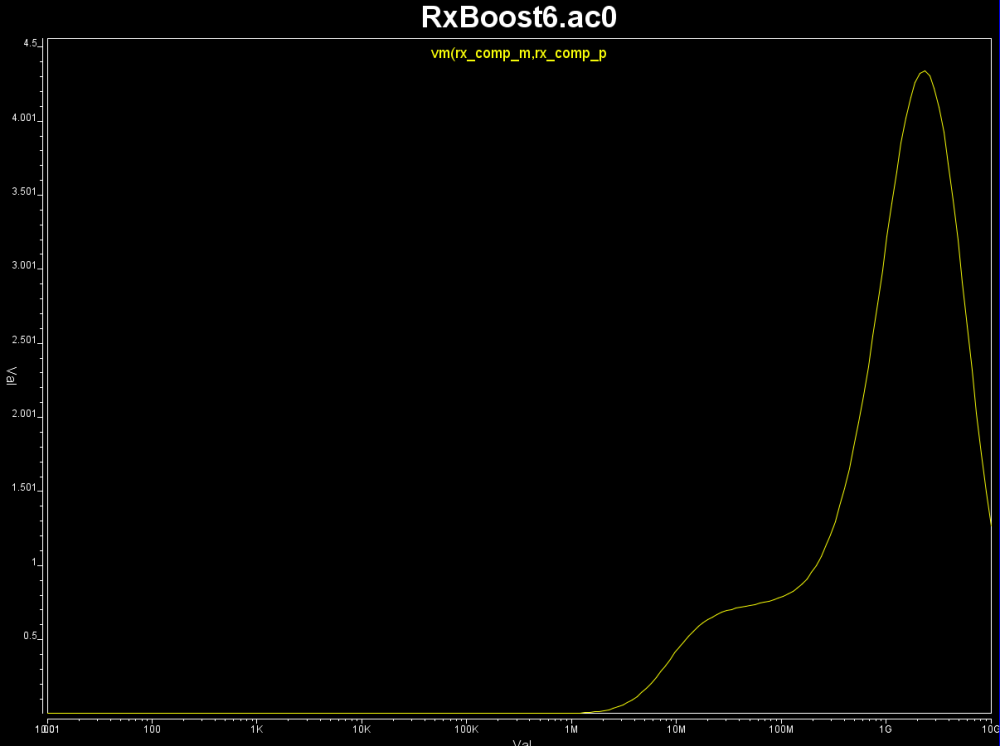
From these eye plot, we do not see DFE like abrupt force-zero output, thus the Rx model seems to be a CTLE like boost filter. So we created Rx test bench like below and obtain its frequency response: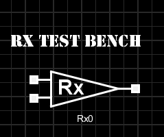
Note that in order to perform what-if analysis of next step, we also use VPro to capture inputs to these Tx and Rx models so that they are evenly spaced.. as required by AMI’s Init and GetWave function. These evenly spaced inputs will be used later on by SPISimAMI.exe to drive the model. For HSpice, the following option may be needed so that the .tr0 file will have evenly spaced data points even simulation is various time-step sized:
- Define architecture:
Now that we have input data and desired output for this particular set of parameters, next step is to explore whether SPISim’s existing spec. model is sufficient to meet the performance.
Tx: for tx module, we observed the following two characteristics:
- Has de-emphasis, happened after the peak
- Swing range and offset are different between input (0 ~ 1) and outputs (-0.5 ~ 0.5). Also there are loading effect so rising and falling have RC charging/discharging like behaviors.
For the de-emphasis part. We can use Spec. AMI’s what-if analysis to see how different pre/de-emphasis settings will cause difference responses:
We change these pre and post cursors one at a time only, using -0.1 for value .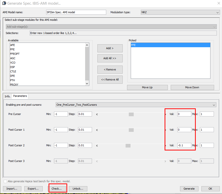
We then test drive using built-in PRBS with same UI time, 200ps: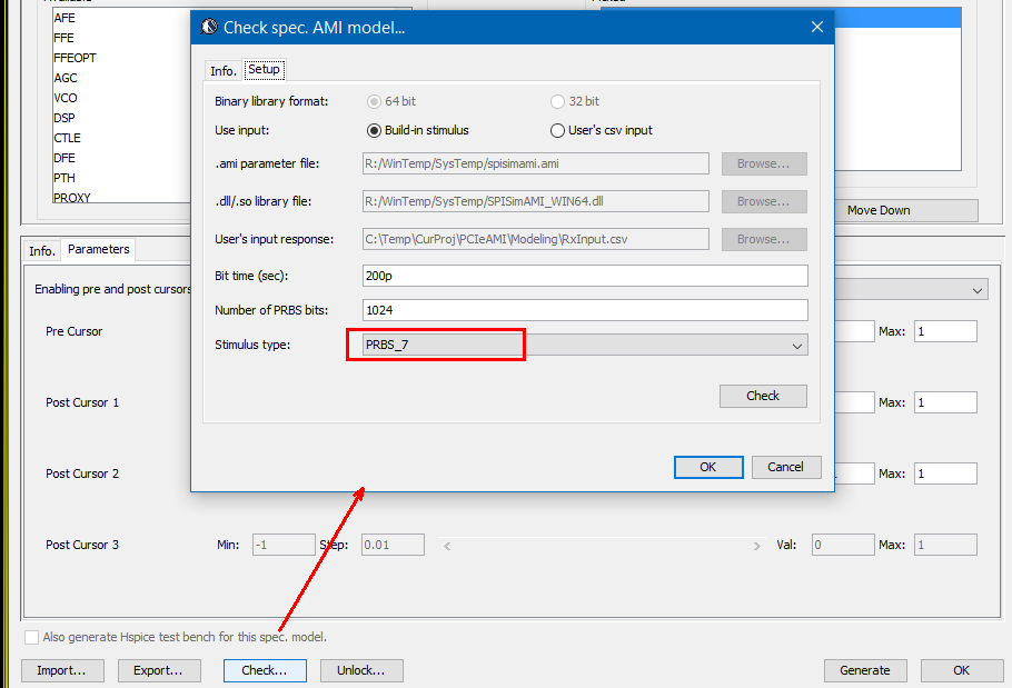
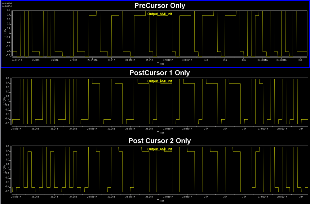
From the summary plot above, and correlate with the Tx output, it’s apparently that this Tx has one post-cursor FFE beause only this set-up gives de-emphasis after one UI after the peak.
For the output swing and slew rate, it’s the sign of AFE (analog front-end). So we can simply add an AFE stage right after FFE, with high/low rail voltage “clamped” to the simulated peaks:
With several trial-and-errors, all within SPISim’s Spec-AMI GUI, we obtained the following Tx correlation between spice test bench and AMI results for this particular set of parameters: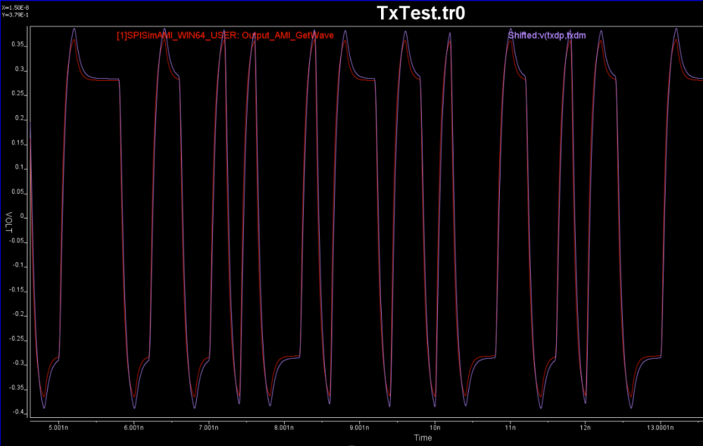
Similarly, as Rx behaves like a continuous filter, we use a CTLE stage to mimic its behavior: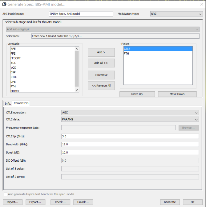
With several tuning, we obtain such Rx correlations: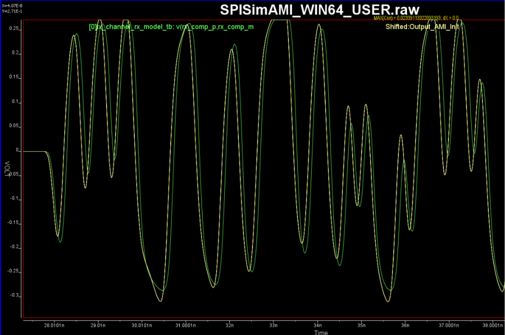
From these correlations, we believe that the stages built-in to the SPISim’s AMI are sufficient to meet the performance needs. So next step is to find the parameters to support all these design specs.
As similar process between Tx and Rx, we will use Tx as an example to demonstrate the flow.
- Simulation/Sweep plan:
Before generating a simulation plan, we first also make sure these design parameters are independent with each other. We performed simple 1D sweep (several points) in particular for the swing and de-emphasis level.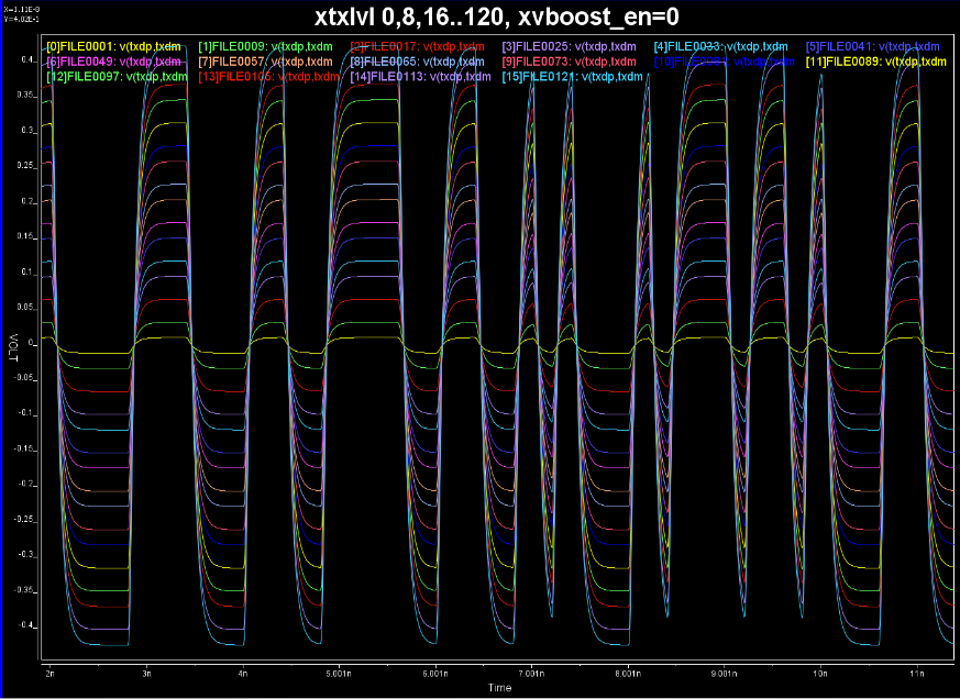

Notice that the slew rate and peaks are not affected by de-emphasis level much. In addition, the spacing seems linearly spaced according to the bit settings. With this, we can sweep them independently.
Now for Tx, a full factorial sweep will require 2^6 (de-emphasis level) * 2^7 (swing level) * 2 (boost flag) * 3 (corner) * 3 (voltage levels) ~= 150000 runs. Due to the linearity, we do no need to sweep full 6 and 7-bits of de-emphasis and swing levels. Instead, we increase step interval for simulation because SPISim’s model’s built-in interpolation can be applied automatically, more about this at the model release section.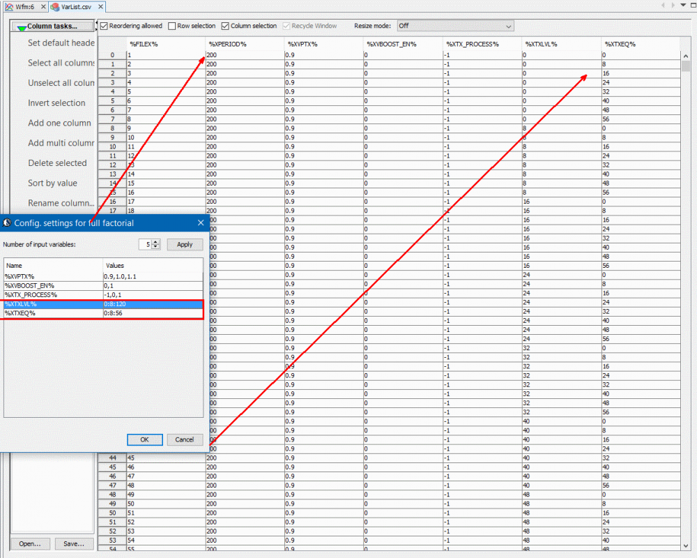
For these five variables, we use MPro to generate 2403 test case (1/60 of full factorial). We then create a template from the Tx spice test bench so that parameters can be updated according to the table and its column header above:
Noticed that variables are enclosed with “%” (e.g. %XVPTX%). Their values are replaced by corresponding values in each row of the table to generate a new spice file. With all these 2403 spice file generated, each for different combinations of parameters, we kicked-off the batch mode simulation and obtained all two thousand cases within one hour. This is done all within MPro and can also be done using user’s script.
- Parameter tuning:
With all results being available, next step is to find corresponding AMI parameters for each of the case. SPISim’s model driver, SPISimAMI.exe, is a must have here. It will take the collected, evenly spaced inputs to drive the AMI parameters together with the SPISim’s spec. model, output results can then be correlated with the .tr0 file simulated with HSPice for that particular case. In case when the correlation is not good, AMI parameters should be updated again for another iteration of performance matching. This process is summarized in the flow below:

Apparently, such as task is too tedious and error prune for a human to perform. Since the input pattern is the same, relative timing locations of different properties (such as peak and de-emphasis levels) are also the same even between different test cases, we can process these data automatically. Regarding “adjusting” AMI parameters, a simple bi-section search will quickly converge to the desired de-emphasis tap values for the given test case.
In our process, we first parameterized the .ami file as shown below. This ami file is based on the architecture identified in the second step… only that now we need to find different values for different parameters. In particular, the swing level and FFE post tap are unknowns and need to be swept.
Because these two variables are independent, we can first identify the peak value as “Swing” from the .tr0 simulation results, then use bi-section to adjust the FFE_PARM_POS1 such that the output from SPISimAMI for this .ami file settings and SPISim’s spec .dll/.so will match the tr0 data.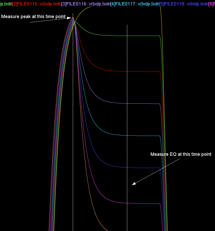
With this flow and process, we use our SPIProcPro to bath process the simulation results and get all 2403 fine-tuned AMI parameters within one hour: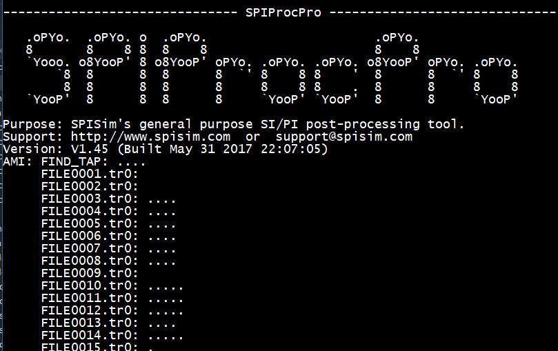
Here is the partial config. settings for SPIProcPro of this modeling process: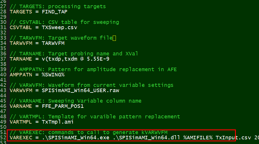
For each of the test cases, the post-processed AMI result is saved to an individual .csv file. All these csv files are also combined and then concatenated side-by-side with original input condition. The end result is a table with input condition at the left and associated AMI parameters at the right. This table will serve as pre-set data table for our AMI models to be released.
Model release:
The combined table looks like below: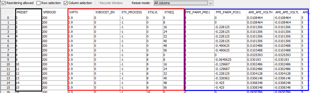
The columns boxed in blue above are those required for SPISim’s AMI spec models. These columns has header named exactly the same as those in the ami file green boxed below. The row entries for settings of each test case in the csv table is filled in to the boxed in red in ami file below.
Now this is not the format to be released to the AMI user. In stead, the design parameter we want to expose to the end user are listed in the red box in the csv table. They have the column headers matching original IP’s design parameters. Also note that this csv table only contains partial results as we didn’t perform full factorial sweep for all ~150000 cases.
The design parameters, boxed in red in csv file, need to be able to be mapped to those boxed in blue, the AMI stage’s parameters.
One unique feature of SPISim’s AMI model is it supports of table look up and up to two dimensional linear interpolation for numerical values not found. The set-up is easily done from model config. GUI. The example below is for PCIe with 11 preset tables.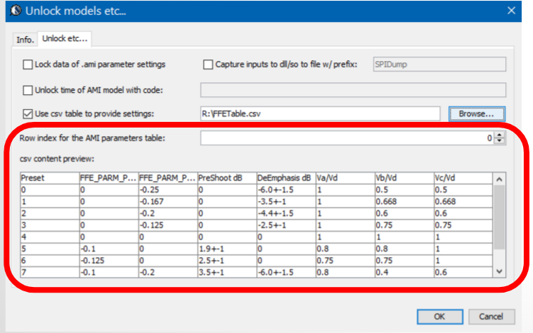
In this case, we do not use preset index. Instead, we set the preset index value to “-1” to signify that model’s table look-up will be used: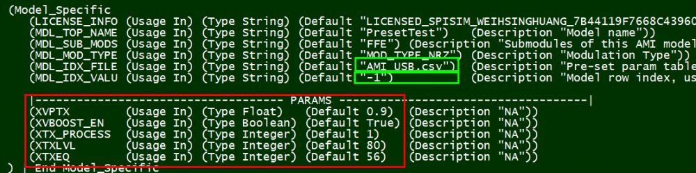
In the final .ami file above, the exposed parameters (boxed in red) are exactly those defined in the original given IP. Their name and values will be used to look-up from the table to find matching row. If up to two rows have no exact match in terms of numerical value, linear interpolation will be performed by the model during initialization. A final matching row or values will be used to assign to the parameters required by spec model.
The final results of the create model is one .ami file, one .csv file (plain or encrypted), and one set of .dll/.so file. There is no need to write any C/C++ codes or even compilation for the AMI modeling purpose and the SPISim’s spec. models can be used directly. For the post-processing portion, a python/perl/matalb scripts can be used instead if SPIProPro is not sufficient.
Other thoughts:
In this case study, a look-up table based approach is used to create AMI model via reverse engineering. Alternatively, we can create a spice simulation session using our SSolver/ngspice spice engine to simulate these given Tx/Rx spice model directly. The pre-requisite for this approach is that the given hspice model is not encrypted, can be converted to the SSolver/NgSpice based syntax and has no process file involved. Regarding search mechanism, a bi-section searching algorithm is used in our modeling process here as there is only one value (EQ variable) needs to be determined. The amplitude/swing is deterministic and can be found once tr0 simulation results is post-processed. If there are more than one variable involved for optimization , such multi-tap EQs, then a gradient descent based algorithm may be needed if full surface sweep is not practical.