Simulate IBIS Data with Free Spice [Q & A]

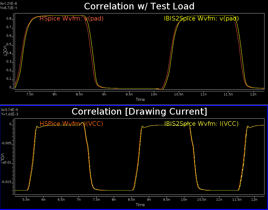
I presented our developed “Ibis to Spice” flow last week at the IBIS summit of 2016 DesignCon. It was well received. In this post, I recapture discussions raised in the Q & A section for those who didn’t attend the summit.

  • Q: Does free spice have IBIS parser?
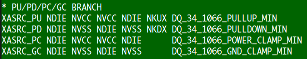
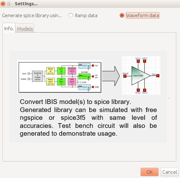
    • A: Nope. Neither NgSpice nor other free spice simulators that I am aware of come with IBIS parser. As a matter of fact, none of the free spice supports IBIS model at this moment. However, interested user may see what pyIBIS has offered and make use accordingly. Lastly, accordingly to the IBIS website, one can pay about $2500 and obtain source codes of golden parser. In our tool, we do have built-in IBIS parser implemented in cross-platform format to support this Ibis to spice conversion flow.
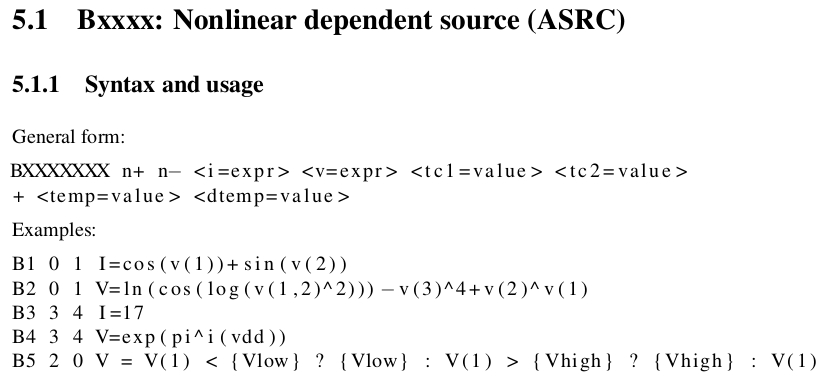
  • Q: Where is ASRC? I can’t find it in Berkeley Spice 3f5’s manual.
    • A: Please try NgSpice instead. Free spice simulator like NgSpice, EiSpice, LTSpice or even TISpice are all Berkeley spice derivatives. Their syntax may be deviates a little bit but the proposed algorithm should work on these simulators with very small syntax changes.
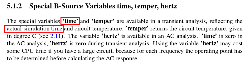
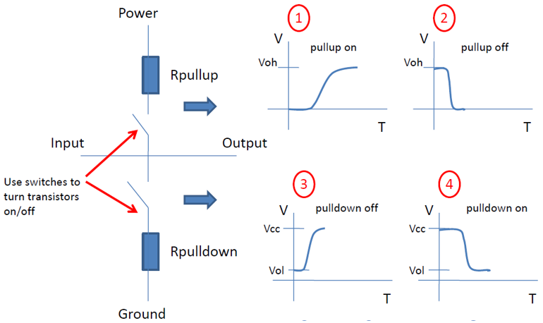
  • Q: Does this template only work for buffer with symmetric rising and falling?
    • A: Not true. The template we have developed will digitize the analog input to a digital one… one with very sharp rising/falling edges. The detection is based on a voltage threshold. So it does not matter whether the rising and falling time of inputs are symmetric or not.
  • Q: Can this spice template account for buffer overclocking?
    • A: IBIS spec does not specify how a circuit simulator should behave when a buffer is overclocked. So the results of a overclocked buffer maybe already circuit simulator dependent. Ideally, a mechanism will make sure current contributed by the pull-up/pull-down branches stays continuous during buffer clocking. This way voltage will also be continuous instead of sudden jump or drop. I suppose a more complicated mechanism can be added to the template to account for situations like these. However, it is not there at this moment.
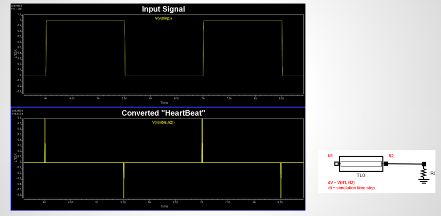
  • Q: Will there be any issue if I simulate the buffer very long, say for 1us?
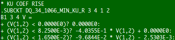
    • A: If the parameter used in ASRC element is too small, for example the original value of time “t” used by switching coefficients, then it will be rounded and cause incorrect results. This is because we usually use ps range as time step. That’s why we scale the value up in the template and also account for for this scaling in the pre-calculated Ku/Kd coefficients. If the scaling is 1E9 (as based line for for 1ns), then 1ps will becomes 1E-3 and 1us will be 1E3, both should not be rounded by the simulator. Thus I think this approach should work for long simulation time, such as 1us.
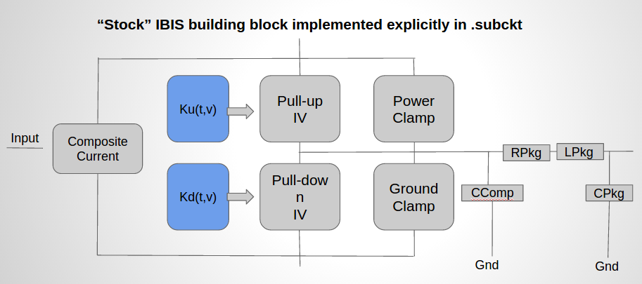
  • Q: Why is T-Line needed? Isn’t it the case that simulator has buffer history which can be accessed for the same reason?
    • A: Yes, most of circuit simulators have a buffer to record nodal voltage history. This way if one decides to use Trapezoidal rule to calculate first derivative, the previous two points can be used. Note that I am using purely spice syntax and element to mimic the dv/dt and delay effect. I have no access to the underlying C/C++ buffer structure, that’s why lossless T-Line is used. With this approach, if one want to get history data of more than one time step before, cascaded T-Line can be used. At each junction of the T-Elements stores the voltage history of previous n time steps (each T-element is one time step delay long).
  • Q: Why is “fine tuning” for handing off needed? Ku/Kd should have reached steady state already before transition.
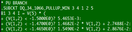
    • A: When buffer is not overclocked, Ku/Kd will reach its steady states. For example, Kur will be come 1.0 at the end of rising transition so that pull-up branch is fully “ON”, while Kdr will becomes 0.0 so that pull-down branch is fully “off”. The reason we need the “fine tuning” to make sure “handing-off” between Kur and Kuf (Kdr, Kdf) is smooth is purely due to the spice syntax based implementation. Theoretically, it’s not needed. User may take the provided template and comment out the “fine-tuning” section and observe the spikes. If you find out other simpler method to filter out these spikes, please let me know.
  • Q: What is next step?
    • A: We plan to continue the path to support system simulation using free spice. Take NgSpice as an example, there are three approaches to add support for a new device, such as IBIS:
      1. Add as a native device like R, L, C: this requires knowledge of circuit simulator algorithm, the code structure and flow. Developer needs to codes in c and extend the arrays of existing device structure. It requires lots of effort and may take longer time to complete.
      2. Add a code-model library using XSpice extension: this requires knowledge of XSpice extension to NgSpice. Developer still needs to code in c still and compile code model as dynamic linked library, but the structure and flow is limited to XSpice device. There is no need to touch underlying spice infrastructure. It’s easier comparing to approach “1”. The compiled library is platform and os dependent, and is a little bit tedious in debugging (need to attach to a running process as the code model is loaded library). However, the developed code model library can run on any existing or released NgSpice simulator.
      3. Use ASRC element to model the behavior outside the simulator: This is what we have accomplished so far. It works well but performance is not that great.

In current version of NgSpice, IBIS, W-element and S-parameter device needs to be added to support system analysis. We plan to continue to approach “2” above and provide support of these devices in the form of  code-model library.

Simulate IBIS Data with Free Spice [Part 2]

Note:

Interested reader of this post may also want to follow up with the [Part 1] of same topic and try out the [Free Web App] which realizes this conversion flow.

For the motivation behind our Ibis to spice development and Ramp based Ibis2Spice conversion flow, please see [previous post]

Waveform based Ibis2Spice conversion:

Typical IBIS model simulation makes use of its waveform data. Thus a converted spice model from its IBIS model must be able to use these timing related data to have good correlations .

Both voltage and current related data can be timing related: In IBIS model of version 3.2 and up, one ore more “rising” and “falling” waveform may be included. Typically, two set of waveform under two different loading condition will be provided. In case only one waveform is available, simulator may convert ramp data to form additional set of waveform. In IBIS model version 5.1 and up, “composite current” is also included in order to account for simultaneous switching noise. This current information is point-to-point aligned with their voltage counterpart to withdraw current from power supply terminals of the buffer model. Note that what we call “timing” here is actually “elapsed time” after buffer’s input signal switches from low to high or high to low. Two sets of switching coefficients, Ku/Kd for rise and fall transition respectively, are used to mimic the gradually turning on/off the PU/PD branches such that under test load condition, the voltage and current waveform data can be reproduced accurately. By using these swtching coefficients, buffer’s strength will be scaled accordingly depending on the load. User may see [our past s post] for buffer’s operation in more details.

Once we have the related  info. then we can create building blocks and assembled exactly as  they are meant to be used in IBIS model, but now in spice format. So the schematic of our waveform based converted spice model will look exactly like a “stock” IBIS:

Selection_209

To achieve this, i.e. be able to use timing data in converted spice model and run like a stock IBIS, three main challenges need to be overcome:

  • Extract “elapsed time” info. during simulation;
  • Compute the switching coefficients Ku(t)/Kd(t) for both rise and fall transitions;
  • Assembled the block together and mimic actual IBIS operation.

Extract “elapsed time” info. during simulation:

In free spice (e.g. NgSpice)’s ASRC (Arbitrary SouRCe) element, function can be used.  One function parameter which may be used for this timing purpose is the “time” variable:

Selection_210

By using this “time” variable, we can calculate and extract the “elapsed time” info.:

  1. First, we need to be able to differentiate between rising and falling from input. This is because both rising and falling transition needs its own Ku(t)/Kd(t) table. After converting input analog to a digital signal, we can use first directive such that rising and falling can be differentiated. To compute dv/dt, a transmission line (TLine) can be used. Other choice may include using a Laplace equation in control element to mimic the “delay”. The decision of using TLine for the delay is also because in free spice, the control element does not support “delay” parameter like other commercial simulator does. Measurement of voltage differentials across TLine gives us dv and TLine delay is a single simulation step dT. TLine is terminated with its characteristic impedance so no reflection will incur at the far end.Selection_211
  2.  Once rising and falling transitions are separated, we can multiply the converted dv/dt with “time” variable and also use a “latch” to hold the signal at the end of the transition. Again, we use a matched TLine as a “latch”: by feeding near end voltage with the far end one, which is data of previous time step, we can have a latch holding signal indefinitely. The latched signal is show in red of the upper plot below. With another “time” variable subtracting this latched signal, we can then obtain “elapsed” time as show in the lower half of the plot. One caveat is that in typical time domain simulation for SI/PI, time step is pico-second range. Spice will ignore variables of very small value, such as 1E-12 scale, thus a proper scaling will be necessary.Selection_212

Compute the switching coefficients Ku(t)/Kd(t):

With the elapsed time, t, now available, we can compute Ku(t)/Kd(t). There are numerous paper and presentation detailing the algorithms. For example, one may compute this switching coefficients from model data based on the first reference below, or use measured based approach based on spice simulation detailed in second reference:

  1. Extraction of Transient Behavioral Model of Digital I/O Buffers from IBIS, Peivand Tehrani et. al, 1996 Electronic Components and Technology Conference.
  2. General K-table Extraction w/ Spice, Bob Ross, IBIS Summit, DesignCon 2015

In general, waveform data from two different test loads are used to solve two unknowns at each time points during rising/falling transition. This calculation is done offline in advance and the resulting data are again realized in the form of ASRC devices. The PU/PD/PC/GC branches will be exactly PWL based ASRC, only that the PU/PD takes one more input (NKUX, NKDX below) which is the switching coefficients, Ku(t) and Kd(t):Selection_205

Ku/Kd are ASRC with pre-computed coefficients and variable of “elapsed time” computed from the first step:Selection_206

PU/PD branches draw associated  current based on the Ku/Kd value presented as voltage value at node 5 below:Selection_207

Assembled the block together in spice formats:

While netlisting different PU/PD/PC/GC/Ku/Kd blocks together is trivial, a nuance becomes apparent during validation: the assembled spice model will have “spikes” right before and after each transitions which makes the model unusable.

Further investigation reveals how devil is hiding in such details… As explained in our previous post, there is a “hand-off” during transitions:

That is, when we “run out of” Ku/Kd for, say rising transition, we keep using the last point data until buffer is about to switch from high to low state. At that point, “hand-off” happens so that Ku/Kd for falling transition will be used. The “hand-off” process is triggered from input and even a time step delay in terms of table usage switching will cause huge spike and cause problem. With carefully looking into different signals in details and figure out their relation in timing, we have a solution which filters out all the spikes and produce a well correlated results, as shown below:

Selection_202

Both the voltage waveform and drawing current matches quite well. The small delay is insignificant because it’s a constant added to each cycle and will be eliminated in the eye plot.

As we introduce two single time step delay transmission line elements to calculate dv/dt and serve as sample-and-hold functions, they also limit the simulation time step a simulator can take. As a result, the converted model run much slower compare to its IBIS counterpart run in other commercial simulator under test load condition. In extracted channel simulation, the “slow down” becomes less apparent as there are multiple transmission line segments present in the topology. The time step limit introduced by the shortest transmission line is common to all simulators which may not be much longer than the TLines we have introduced.

Another note worth mentioning is that while this post focuses mainly about Ku/Kd and voltage waveform data, Composite current and their ISSO_PU/ISSO_PD are treated similarly: An ASRC constructed from composite current based on time aligned point with voltage counterpart is used to draw current. Another set of scaling table, based on ISSO data ares computed off line in advance in order to take the non-ideal voltage supply into account.

With both ramp and waveform based Ibis to spice flow being available, we are able to perform SI/PI simulation using IBIS on free spice simulators. Such flow has been integrated in our SPIBPro flow as shown below:

Ibis to Spice function is SPIBPro

Ibis to Spice function is SPIBPro

This post is written in preparation for the upcoming IBIS Summit at DesignCon 2016, where we will present this Ibis to spice flow. The presented slides and associated examples are shown below. Reader may also download them from IBIS's official page for this summit.

Presented slides: View externally [HERE]

Example files: [click to download]

Simulate IBIS Data with Free Spice [Part 1]

Note:

Interested reader of this post may also want to follow up with the [Part 2] of same topic and try out the [Free Web App] which realizes this conversion flow.

IBIS to Spice:

Most of the buffer modeling flows focus on creating IBIS models from existing transistor buffer design, usually in spice format. However, we also find values in  flow of doing the other way around, namely converting IBIS model to spice format. This is motivated by one or more of the following reasons:

  • System SI/PI analysis support with free spice simulators: There are several simulators, e.g. Berkeley 3f5, eispice, ngspice, LTspice, available in public domain or free of charge. Due to historical reasons, their focus tends to be more on-chip or vendor products specific, like BSim3/4 for Berkeley spice and voltage regulator for LTspice. While they all have certain degree of transmission line support, yet when it comes to IBIS portion, they are totally lack of. Without driver model, which usually comes in the form of IBIS models, one can’t perform system analysis! It’s certainly possible to develop native IBIS support into these simulators, but the immediate available solution is to have a flow to convert existing IBIS model into sub-circuit like format and be able to simulated in these simulators. The added benefit of this approach is that engineer who has ad-hoc need to run SI/PI simulations with IBIS involved can do so quickly with these free available simulators without incurring much overheads.
  • Vendor neutral release of IBIS reference data: IBIS is a non-proprietary data format. When implemented correctly, simulation results from different simulator vendors should correlate with each other very well. To help achieving this, “golden waveform” data can be part of the IBIS model release. In reality, the “golden waveform” is optional and each simulator vendor’s implementation is different, thus the results may be different. We have seem model providers, such as Micron etc, also provide encrypted hspice as part of  the release to provide “golden reference” for the IBIS model. The disadvantage is that encrypted model needs to be run on proprietary simulator which is usually not free. So there is a value to be able to release IBIS, its corresponding data in non encrypted form AND allow user to validate the model with public domain simulator as well. This also encourages (simulator) vendor neutral model release.
  • Explicit IBIS algorithms implementation for educational purpose: There have been many papers and presentations detailing usage of IBIS data inside a circuit simulator. While it’s good for high-level overview, the truth is that these algorithms are often implemented deep inside a circuit simulator. With the developed Ibis to spice flow, we expose these algorithm in the form of plain text (versus C/C++/other programming language) spice compatible subckt format. We believe it will  be very educational and have much reference value.
  • Speed up flow development: Circuit simulator is one of the back-bone of SI/PI analysis (field solver can be one of the others).  To be able to use simulator as part of the developed flow, several options are possible: 1. choose to work with established simulator vendor and require customers to have license accordingly, 2. develop one internally, or 3. make use of tried and proven ones in public domain. Each of these approaches has their pros and cons. As a start-up company focusing on providing flows of high C/P (Performance/Cost) value, we would like to save the cost of other licenses and development efforts for our customers and speed-up the development when possible, thus option 3 is a very attractive solution to us.

There is already a vendor providing Ibis2Spice in their tool. Their free version supports only up to V2.1 IBIS model and the paid version only up to V3.2 IBIS model. Having that said, the model converted by their tool can’t be simulated in free spice directly. The flow we have developed can supports up to V5.1 model which includes the current information like [ISSO] and [Composite Current] keywords. In these two posts, we will explain about our flow in details. We will first review how ramp rate data can be used in free spice, followed by how waveform data can be converted into spice, accompanied with correlation data in both cases.

Goal of developed flow:

  • Run on free simulator, e.g. Spice3F5 and NgSpice
  • Support VT waveform data (IBIS V3.2 and up) and current data as well (IBIS V5.1 and up)
  • Produce very good correlation compare to commercial IBIS implementation.

Ramp based Ibis2Spice conversion:

In this first post, we will review the existing Ibis2Spice flow. We have also re-implemented this IBIS to Spice flow and release it free in our SPILite module. Output from our flow is directly usable in free NgSpice, which is also included in our tool. Basically, it uses ramp rate data only in the given IBIS model and creates a corresponding spice model. The learning here is how behavior source, ASRC (Arbitrary SouRCe) can be used to implement the IV table lookup. This technique will be applied more extensively in waveform based Ibis to spice flow (next post).

Searching from the web will bring you to this post (for original author’s credit): IBIS to Spice Translation (part 1). In this post, author describes the operation, his attempt to modified circuit and the result. He also provided an Awk script to accommodate the the changes needs to be made in order to run on free spice. As this post is written more than twelve years ago, part of the content has been outdated. For example, the NgSpice 26 does accept the syntax like  X + -3.12 so there is no need to convert to X-3.12 any more.

The part 2 of the original post show the schematic of the converted ramp-based spice circuit. It is hard to find on the web, so we post it below to save reader’s effort:

Ibis2Spice Schematic

The key elements here are four IV curve data: XPWRCLAMP, XGNDCLAMP, XPULLUP and XPULLDOWN. These four IV tables from original IBIS have been realized with ASRC sources, as explained in NgSpice manual:

Selection_195

The power clamp and ground clamp branches are always on, so the data is used directly. Their ASRC data is a converted PWL curve shown below. Depending on terminal voltage V(1, 2), current will be output or drawn from terminal 3 and 4.

Selection_199

For pull up  (PU) and pull down branches (PD), they are turned on/off only after buffer has switched, the rate of turning on/off is based on a RC constant (C1 and RB3 in the upper left of the schematic) converted from ramp rate value in the model. This RC value is then used to multiply the PU/PD voltage and finally converted to a current source using G element (VCCS, Voltage Controlled Current Source).

Selection_197

Selection_198

In the original post, author mentioned he has attempted to replace this RC based implementation with his PWL version yet get non-smooth results. We think this is because PU/PD branches are turned-on/off gradually. Only when they are left for certain period of time, static state will be reached. Thus a “time” based parameter must be present. Otherwise, static solution is solved at each time step and thus result will be incorrect. RC multiplier realizes this transition of “gradually” turning on/off the PU/PD branches.

With the RC based implementation, one can mimic the “ramp” data used in other IBIS capable simulator and produce good correlation, as shown below. Due to the simplicity of this implementation, the simulation speed is very fast.

Selection_201

Note that with this implementation, drawing current from VCC/VSS are way off. This is also indicated in the original post. As a result, this approach will not be useful for SSN simulation which includes PDN noise. Further more, it will not capture initial undershoot, final overshoot and other more subtle waveform presented in real buffer switching, also the RC curve (shown in the red above) is not true “linear”. In additional to the ASRC based implementation for IV tables explained above, part of the converted circuit is used to detect and convert input analog signal into digital ones. Lastly, each corner of the model to be used in the simulation needs to have a spice subckt library converted from corresponding corner in original IBIS model.

This post is written in preparation for the upcoming IBIS Summit at DesignCon 2016, where we will present this Ibis to spice flow. Please see the [Part2] and download presented slides and associated example files.