S-Param: Analysis report

Preface:

A S-parameter model can be obtained from lab measurement using VNA, full-wave field solved from a 3D structure, analytically computed via AC simulation or analysis process such as cascading of various stages. There are many situations when more than one s-parameters will be generated for similar setup. When dealing with multiple s-parameters, one should be able to quickly batch process and generate a summarized report for desired performance or measurements. Equality important is to be able to investigate and debug on a case by case basis. Both of these functions are also must haves for an EDA tool supporting S-parameter models.

Example report from the PLTS tool

In this post, we would like to discuss points of considerations when planning for these types of analysis and reporting capabilities. We would also demonstrate how they are accomplished in our SPIPro tool. Most of the mathematics for these processing can be found on website such as RFCafe or matlab RF toolbox.


Analysis:

There are many analyses often used so far as s-parameter is concerned.  They can be classified into several categories:

  • Conversion: such as converting a single ended S-parameter to a differential one or one with mixed mode (mixed single and differential), converting between S and Y, Z, ABCD formats, etc
  • Extraction: such as trimming unwanted frequency data points, extracting subset of S-parameter, or calculating physical properties such as impedance, effective inductance etc
  • Generation:  such as cascading different stages together, either assuming generalized 2N port in a point-to-point topology, or arbitrary ports branching out like those multi-drop situations in DDR, combining S-parameter data in other fashions such as merging, synchronizing frequency samples etc.
  • Processing: such as smoothing the data using moving average, extrapolating toward DC and high frequency based on physical properties, renormalizing reference impedance to different values.

10 of 30 SPIPro’s S-Param analysis capabilities.

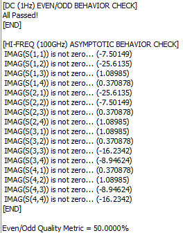
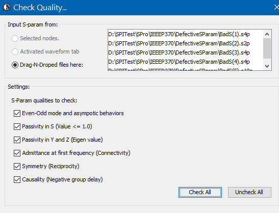
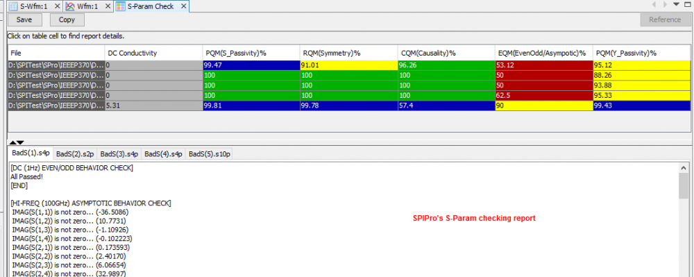
Based on our experience, Convert, Cascade, Renormalization and Quality check are most frequently used. For mixed mode conversion, several port ordering scheme should be supported: incremental, interleaved or even-odd mode.

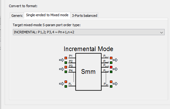
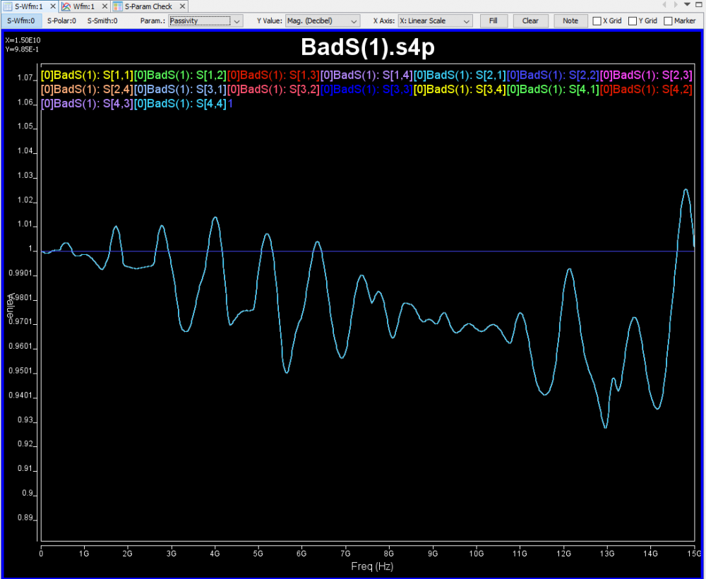
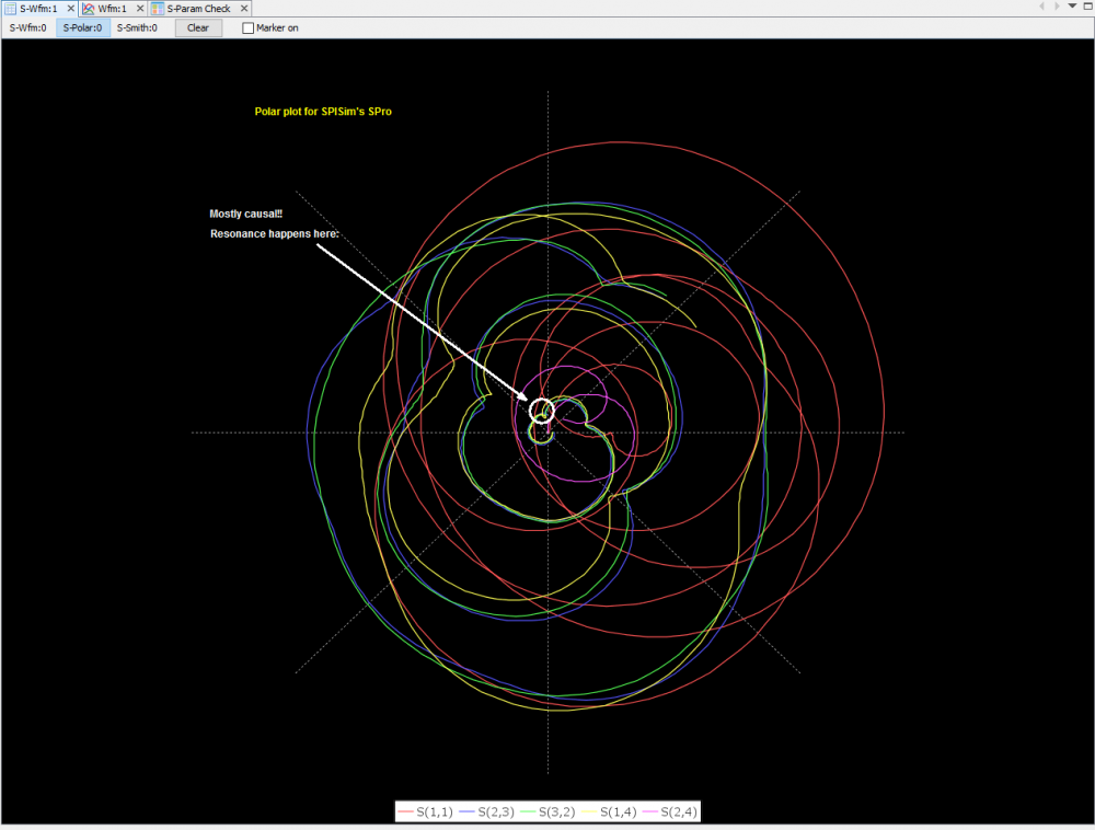
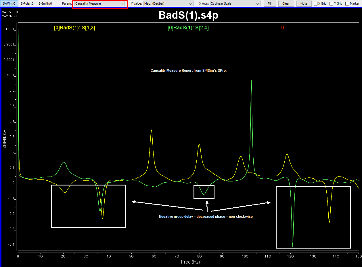
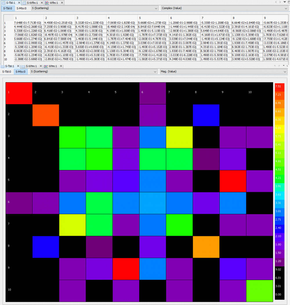
The outcome of the processing above are mostly another s-parameter. Thus one should be able to inspect selected individual Sij element either visually or textually further. For the same set of data, it can be plot in different format to reveal different properties or behaviors. For example, X-Y format by default, polar plot for causality inspection and smith chart in either Y or Z format etc. Since only several Sij elements are plot instead of the full S-parameter, some analysis can be done almost in real time to provide feedback: time domain reflection (TDR), time domain transmission (TDT), worst case eye analysis based on pulse distortion analysis or even passivity plot etc.

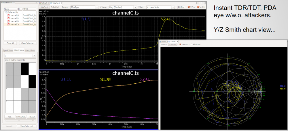
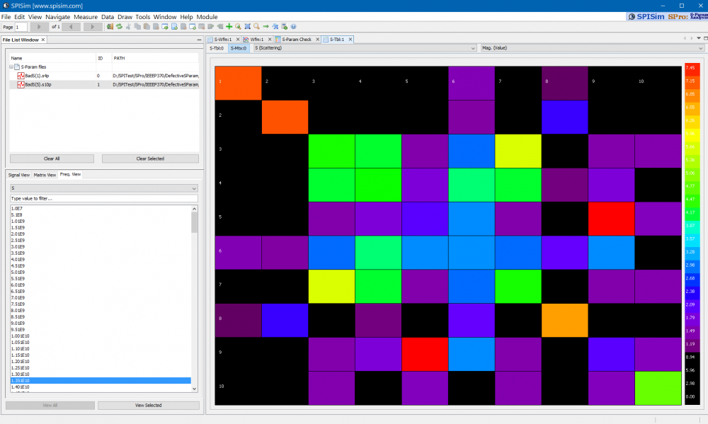
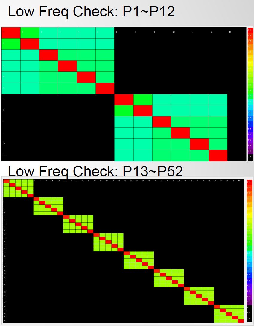
Texture representation can be useful when one needs to copy part of the calculated data for further analysis, such as taking effective inductance for power integrity simulation. Color coded matrix at the first and last frequencies are also useful for quickly checking connectivity or high inductance ports.


Report figure:

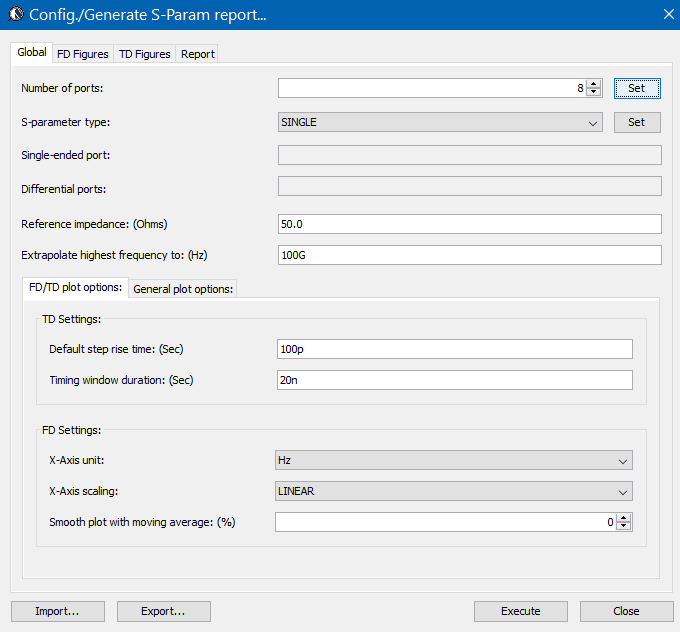
The analysis process mentioned above are good for investigation or experiment purpose. When there are more than several s-parameters need to go through similars sequence of operations, being able to batch process and report becomes important. In this case, the input conditions such as number of ports, their mode (single ended or differential etc) port ordering and reference impedance etc are specified up front (via GUI or a template). This settings will be applied to all the given s-parameter such that after they are read in by the tool, this sequence of actions will be performed automatically. After calculation,  report in the form of various figures, statistics and csv can be generated:

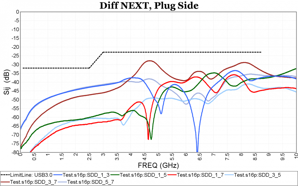
  • Frequency domain figure: one or more selected Sij traces from the processed data can be plot in the X-Y chart in linear or log scale. Waveform calculation using real or complex number with various operator including log and power should also be supported. Multi stage limit line can be added to identify boundaries which signal traces should not cross.

One or more such figures can be defined for different data and measurements.

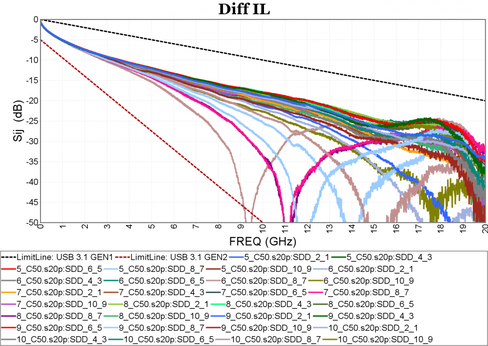
  • Time domain figure: For time domain, Sij needs to be converted using iFFT first. To achieve certain time domain resolution, extrapolation to higher frequency and data smoothing using moving average may be needed. There are several time domain metrics often used: TDT, TDR, crosstalk, inter-pair and intra-pair skews etc. Input pulse’s rise time may affect the resulting slew rate so it needs to be part of the settings. 
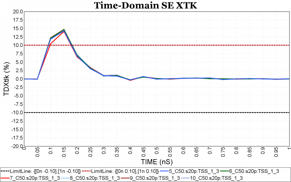
Again, one or more such time domain figures can be pre-configured so that their settings will be applied to all s-parameter data.
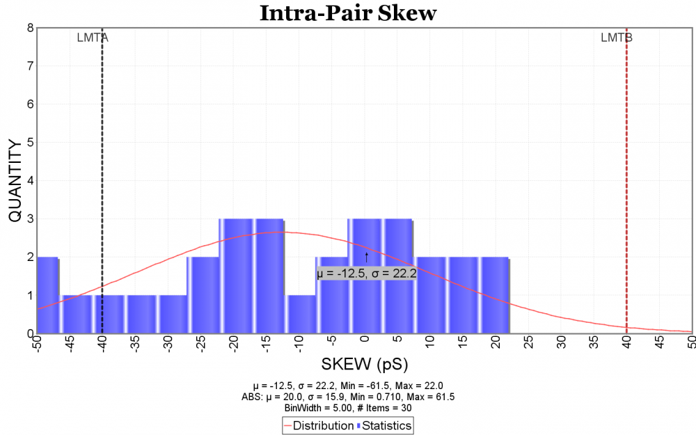
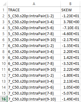
  • Statistics figure: The timing or skew measurement can be summarized using a histogram with distribution curve. Their data in csv format can provide more detailed info. for individual cases.

Allowing further customization such as various font size, frequency unit, grid line etc will make the generated reports more appealing aesthetically. Finally, these settings should be allowed to be imported or exported for later use. Resulting report can be in html or pdf format with indexing at the top of the page. With this kind of capability, analyzing a set of s-parameters become easy and efficient.


Report data:

When there are even more s-parameters to be processed, such as hundreds or even thousands of cases from analysis methodology such as design-of-experiment or multi-dimensional sweep, even visually check with reporting becomes time consuming. In this situation, batch processing to extract performance value, summarized in a multi-column csv fashion to be used for statistic tool such as our MPro or JMP is more practical.

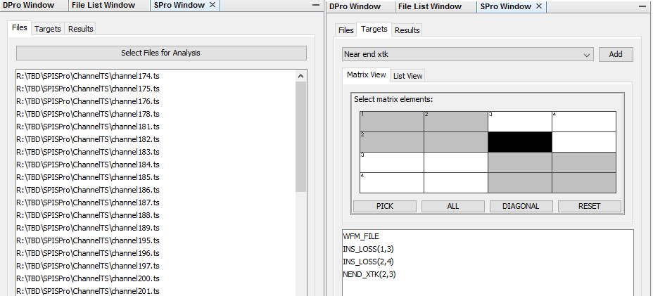
User first specify all the files to be processed, then specify one or more time domain or frequency domain performance targets. The processed results can be visualized as a summary plot. Interested cases or outliers can then be selected to generate more detailed report or investigate individually.

Unless specified, all the screen captures used in this post are from our SPIPro product. All the mentioned functions and capabilities are also supported in this product.

S-Param: Quality checklist

Preface:

In a typical system, there are usually three type of models involving in simulation or analysis:

  1. IBIS/IBIS-AMI: At the both ends of the channel are driver and receiver models, usually in the forms of spice, IBIS and/or AMI.
  2. RLGC: Interconnects with homogeneous structure such as transmission line and/or layer stackup are usually 2D/2.5D field solved and represented with frequency dependent RLGC matrices
  3. S-Parameter: Complicated passive structures such as package, connector or via must be solved with full-wave simulation to have accurate representations, which are almost always S-parameter.

In the recent years, due to the popularity of link analysis for low BER requirement (i.e. various SERDES interfaces), S-parameter has become more and more important. A s-parameter is now often used to represent the full channel (package + t-line + via + connector etc). In addition, there are lab measurements from VNA which are also in the form of S-parameter. Even when behavior models (broadband spice circuit) of these components are used for time domain simulation, they are also converted originally from S-param via algorithms like rational fitting.

Each of these S-parameter may have their own noise sources, bandwidth limitation or numerical inaccuracies. As a result, one has to check the quality of the S-parameter models to avoid numerical errors or instability (e.g. simulation convergence) of the analysis at the later stages.

There have been several documents floating on the web discussing about checking list for a given S-parameter, albeit lack of systematic approach or industrial support across different vendors. For this purpose, IEEE P370 committee was formed in 2015 to discuss and define a spec. as a reference. Task group 3 of this committee focuses in particularly on the S-parameter quality check. As a participating company in this joint effort since the very beginning, also as the spec. draft is coming into shape at this moment, we think it’s a good time now to share the collective thoughts and also demonstrate how these ideas are implemented in tool like our flag ship product, SPIPro.


S-Parameter quality check:

A S-parameter checking list can usually be classified into two categories: generic check and application specific check. This post focuses on the generic check, which is defined as checking based on their physical properties. For the latter one, application specific condition such as signaling speed, typologies, modulation method or even coding are further imposed. Generally speaking, there are several generic checks need to be done:

  • Passivity: to make sure data is passive and has no amplification
  • Causality: to make sure properties of cause and consequence are maintained
  • Reciprocity: to make sure data is symmetric
  • Even/Odd/Asymptotic behavior: to make sure even and odd behaviors are maintained at both DC and high frequencies
  • Connectivity: to make sure connectivity of structure extracted is correct and has no broken link(s)

In addition, reports from all of these check should be presented clearly with an overview and further details available. The overview summary should also use a single number for each check as well as quality metric coded with color for different level:

  • Good: Green
  • Acceptable: Blue
  • Inconclusive: Yellow
  • Bad: Red
  • NA: for information only, such as connectivity

Numerical criteria for these levels depends on the types of check. Lastly, visual checks should also be used in some cases to provide frequency specific information such as where the issue happened.

Full mathematical details and explanations of the sections below will be in IEEE P370 spec.. It will be made available free to public upon completion. We will not duplicate the details here but only giving high level description and demonstration usage below.


Passivity:

Power injected into a S-parameter, which includes those from incident and reflected waves, should be preserved without amplification. When this is true, then S-parameter is passive and does not contain any energy source. Mathematical requirement is:

Visually, we can plot the given traces (Sij) and see whether they cross threshold of 1.0:

And/or compute a summarized metric, Passive Quality Metric (PQM):

reported as a single value:

One way to fix a non-passive system can be use the largest (violated) value to normalize the rest such that no value is larger than 1.0, thus passive.


Causality:

Causality check is the most important, yet more complicated one for a S-parameter. A necessary but non sufficient condition of being causal is that the even and odd function behavior of the real and imaginary data at DC should be satisfied. Adding being passive across full frequency range will make the condition sufficient. So a causality check essentially includes many of the other checks needed for a s-param.

Due to the complexity of the math, such comprehensive check is not easy. As a result, a visual check (heuristic) may be used. This check is based on the observation that a polar plot of a causal system rotates mostly clockwise and is often very smooth. The small inner circle is usually where resonant happens which may degrade the causality of the overall data:

The progress of phase between two adjacent vectors (Sf0, i, j to Sf1, i, j) can be calculated and normalized with their dot product and magnitude. The results should be a value falling between -1 ~ 1. Negative value represents decreasing group delay and thus a counter-clockwise phase change between these two vectors. This is where resonance has occurred. One can plot such measure against each frequency and got its visual representation:

Often time, through type traces of a given s-parameter (S12 or S21) are used for iFFT for corresponding pulse or impulse responses. One can calculate this for each frequency of each through through type signal and have a summarized metric: Causality Quality Metric (CQM)

And report can contain more details about violations of different frequencies:

The fix of a non-causal system usually involves reconstructing a causal system with parameters fit the given data. Vector fitting or rational approximation are such approaches, which will be discussed in future post in more details.


Reciprocity:

As a s-parameter is passive, it should not be directional regarding input and output ports. Thus a S-parameter’s content should be symmetric across the diagonal part. Note that this may not be the case for materials which has non-diagonalizable property such as ferrites, yet it should hold true for most of the materials used in system elements and materials.

For a large multi-port system, color coded cell values can be used as a visual check for symmetry (reciprocity):

This needs to be done at least at the first (low) and last (high) frequency content. Regarding an overall evaluation, a Reciprocity Quality Metric (RQM) can be used:

A reciprocity violation’s fix is usually the easiest… one may average values from both sides of diagonal and replace in place.


Even/Odd/Asymptotic behavior:

This check is based on the fact that a transfer function should be equal to its conjugate in the negative frequency domain:

As a result, the real part of the data should be an even function while the imaginary part should be an odd one. That means at the dc level, the real data should be flat across freq = 0 axis while the image should cross origin point. Also at the highest frequency, the imaginary data should approach zero. One can think of all the inductive and reactive elements such as capacitors and inductors are either open or short at the lowest (DC) and highest (infinity) frequency point, thus make the transfer function real only.

This even/odd/asymptotic behavior is very useful when the extrapolation toward DC and highest frequency points are needed, such as the case for TDR/TDT from iFFT. DC point in frequency domain will affect the corresponding DC value at the time domain, while the highest frequency available will decide the resolution in the converted data in the time domain.


Connectivity:

This is to make sure the structure the s-parameter extracted from does not contain any broken channel. A simple conversion of S-parameter to Y or Z parameter and check their value should reveal the connectivity. Usually doing so at the first data point (low frequency) is enough. Color coded matrix value again will be very useful especially for large s-parameter matrix:

The example shown above is for a full DDR byte lane which involves many DQ and a pair of DQS signals. As DQS is differential, it may also be useful to separate them from the rest of the data with proper scaling for better distinction.


Report and summary:

To apply these checks to more than one  s-parameter, a batch mode process is often preferred and will save lots of mouse clickings:

The produced summary should contain with color coded cell and various quality metric number, plus further details for each check of different data. This will certainly gives user better idea about the quality of their s-parameter files.

All the screen captures used in this post are from our SPIPro product, which also implemented all the checks according to the IEEE P370 spec. draft.


IBIS-AMI: Analysis using a proxy class

Preface:

A hot topic in recent years about IBIS-AMI is co-optimization through back channel. During this process, either Tx, Rx or both participate to select optimized set of parameters in order to have best link performance. The IBIS spec. as of today does not support this type of communication or data exchange between models, thus new protocols have been proposed. In addition, there are also occasional needs to support 1. simulator or AMI models from other vendors, 2. implemented in different AMI-API spec version, or 3. written in different languages such as matalb. Most of these cases, only their binary formats rather than source codes are available. To overcome these obstacles and bridge the gap, a proxy class based approach is proposed.

This post is written in preparation for the presentation of the same topic at the IBIS Summit during DesignCon 2017 on Feb. 3rd. Audio recording of the presentation and slides have been made available at the bottom of the post.

Roles in an AMI flow:

Readers of the latest IBIS spec. will find that Chapter 10, Algorithmic Modeling, is all about defining two roles in an AMI flow and how they communicate through API. These two roles are 1: EDA tool (usually circuit simulator) and 2: one or more AMI models being simulated. AMI API is defined such that EDA tool knows where the .ami file is and which functions are available in the model .dll and can be loaded. In the current spec., no interaction between different models is possible.

Take the .ami file above as an example, the EDA tool is responsible for parsing the ami file and do type and range check first. It then needs to figure out that an “AMI_GetWave” function implemented in the model since the parameter “GetWave_Exists” is set to true. In addition, the waveform process should happen in the AMI_GetWave” call rather than AMI_Init because “Use_Init_Output” is set to false. Beyond this, the only thing EDA tool needs to do regarding “Model_Specific” keyword section is to parse these data and form key-value pairs before passing into model. The simulator itself doe not need to know what they are and how they will be used.

When a break point is set at the function call inside the model’s .dll/.so, one will find that the parameters now form pairs already and can now proceed to consume these settings. Note that this breakpoint will only be hit if the APIs are implemented correctly (thus can be recognized by the simulator and loaded according to the spec.)

With the introduction of the back-channel interface (BCI), new AMI APIs are being defined to support communications between models themselves:

Interested reader can find BIRD147.,1_Draft on IBIS website fore more details. Simply speaking, models can pass data back and forth through this protocol via files. Since this is a reserved parameter, this BCI parameters should also be supported by the EDA tool.

Reader keeping track of this topic probably knows that for the past several years, several EDA companies have been arguing about how these back channel communications should be implemented. Some of the main considerations include:

  • In case when legacy models can’t be re-compiled, how are they going to participate in the optimization process
  • Whether or not a simulator should perform solution exploration actively or should leave this to the models themselves
  • Should the communication protocol be only between models involved or it should also be part of the defined spec. as well

On top of these, we would also argue that:

  • As a simulator/EDA tool developer, how can I test the AMI models at hand for co-optimization?
  • As a model developer, my EDA tool may not be updated or up to date. How can I test the co-optimization if I want to add such support my model?
  • As a model/EDA tool user, can I inspect what’s going on between simulator and models? I only get post-processed results from EDA tool and they are not correct!

For these purposes, we think that a proxy based class can be used in AMI analysis flow.

A proxy class:

The proxy pattern’s UML is shown above. The dot line at the top represents “has a” relationship while the solid vertical arrow line represents “is a” relationship. This UML diagram can be read as: A client has one or more subjects which implement interface function called “DoAction”. When the proxy class’s DoAction is called, it delegate to RealSubject’s DoAaction” function.

Put this in the IBIS-AMI’s context, the statement above can be read as: An EDA tool can load one or more .dll(s)/.so(s) which implement AMI-API’s interface such as AMI_GetWave etc. When the EDA tool calls a proxy’s AMI-APIs, this proxy object delegates calls to RealSubject (i.e. real model)’s AMI-APIs for data processing.

So this Proxy class is a “wrapper” around real model. It’s loaded by the EDA tool yet itself also load the real model’s .dll(s)/.so(s). It’s a “man in the middle” and can be used to intercept, modify input/output data or even perform customized analysis flow beyond what a simulator can do.

In the example above, the proxy’s AMI_Init function loads the model’s dll, identifies the AMI_Init function and then delegates call.

With proxy class, there are several experiments/test can be done:

Consistency/Stress test:

In this example, a model’s functions are called many times. The purpose is to test:

  • Consistency: i.e. when given the same data, will the model return the same result? This should be the case for LTI model.
  • Stress: will there be resource leak such as memory usage keep  increasing?

As mentioned in the IBIS spec, an EDA tool may break up lengthy bit stream into several chunks and call AMI_GetWave many times, thus a well behaved model should pass these two tests.


Co-optimization (internal):

The second experiment is to bundle Tx and Rx’s response together within one function call and try to do something with it (such as iterate to find combinations for best performance, i.e. optimization)

First, from the IBIS spec., or diagram shown above, Tx’s response will be computed first. Most of the Tx’s processing is LTI and its function is mainly to convolve signals with 1 or 4. After this step, EDA tools convolves again with signal 6 before passing on to 7.

Now convolutions is a commutative process, meaning the order can be exchanged:

So if we use a proxy class in Tx’s place and implement a delta response (e.g. simply return the data passed in), then EDA tool will convolve step 4 and 6 as before while we can combine the actual Tx model’s function with Rx together after that and get the same result:

However, these two models are now put together with the Rx proxy’s AMI_GetWave function call. So we have great control by manipulating the models’ pointers directly. This way, setting such as CTLE’s curve index and/or sweep the number of taps and their weights on the Tx side can be performed. This example also demonstrates how a proxy class can intercept call from EDA tool and perform customized flow.

Co-optimization (external):

In the two examples above, data execution is within the same process where the proxy and/or model’s .dll(s)/.so(s) are loaded. However, it’s also possible to implement these in separated process, or on different machine over the network. The diagram below shows an example:

In this case, we want to use EDA tool’s post-processing capability to obtain performance matrices such as eye-width or BER. However, we would also like to adjust the model’s parameters continuously in order to obtain best channel performance. The EDA tool can be called repeatedly, each time the AMI_Init or AMI_GetWave is called by the simulator, a proxy class intercepts and delegates the call to a remote process via communication such as file based IO, socket or shared memory. The remote process is persistent and can be considered as a server. It will return the data back to proxy class upon completing processing, wait until EDA tool’s post-process and updates results, then read and adjust the settings for next call from another simulator run. On the “server” side, a simple AMI test driver loading similar proxy class can serve as the stand-alone, persistent process.  This way all the .ami processing can be done up front by the model driver and no simulator license is needed.

The shaded block in the middle execute socket communication to get response from a remote process.

Other possible uses of the proxy class:

In addition to the examples discussed above, an AMI proxy class may also serve:

  • As a wrapper class to support model implemented in different language, such as matlab, octave, perl etc in either AMI-API compatible library form or executable
  • As a server to centrally manage the SERDES models, provide extra IP protection as it can now sit on some server always updated without being distributed.
  • As a wrapper to support legacy models by implementing support of new spec. or parameters at the proxy level without re-compiling the old models.

We have used such proxy class in our AMI analysis and find it very useful. We also expect it will be even more widely used as AMI models become prevalent and IBIS spec. being updated to support new protocol/parameters.

Materials:

Click [HERE] for the audio recording of the presentation.

Click [HERE] or visit ibis.org for the pdf of the presentation.


IBIS-AMI: Modeling architecture study

Preface:

In previous post, we discussed several possible roles involving IBIS-AMI and their points of considerations. In this post, we would like to focus on the AMI model developer’s role and explore several modeling flows along with their pros and cons. The materials and example discussed here are from publicly available sources and articles, which are also listed at the end of this post.

IBIS-AMI models:

Regardless how sophisticated a SERDES design is, at the end of the day, the work of generating a corresponding AMI model is to create the following the 3 ~ 5 (depending on IBIS spec. version) AMI API functions in C language and compile them as .dll(s)/.so(s) across different platforms and OSes. Noted that the actual implementations (how the SERDES or EQ operates) are not bounded by C/C++ language. For example, one may use matlab, octave, perl or other language to implement the core function, only that they have to be wrapped with C AMI-API functions. Regardless, the main objectives are still the same: translate the design to corresponding codes. On top of that, one also needs to consider how to debug, maintain and extend the generated models for model users and future design revision.

IBIS-AMI API functions

A very popular, and relatively easy approach to achieve this goal is to use tool/program to generate codes directly from design collateral.

Top-down AMI modeling flow:

A typical design flow is usually top-down based: floor plan is made and functional blocks are defined. At first, only abstract level behaviors, budgets and/or spec. are given. Each designer or team then dives into the detailed implementation of these functional blocks and finally assemble them together for full design simulation or verification. Using this approach, a schematic is usually used for design entry and connect different block first, each block may have several hierarchies. Architecture codes/schematics are translated to C/C++ by machine.

User also usually can right click on each block to specify parameters for customization or exporting. When it’s done, an add-on module will translate this design to corresponding C/C++ format most of the time. So far as AMI API is concerned, a special AMI kit may be also needed such that generated codes will be AMI-API compatible.

With this approach, user focuses on SERDES design rather than the coding or API details. Since these architecture blocks/codes are pre-generated and verified, the generated codes are considered well tested and should produce good correlations.

Machine generated codes:

While machine/program generated codes are pre-tested and usually very structured, it may not be easy to debug and extend. While it’s certainly possible to rewrite part of the codes for fine tuning or customization, one should not forget that next time when the designer click “generated c/c++” button again, all the changes will be overwritten. So the update made at the bottom (i.e. generated codes) will not back propagate or back annotate to original design. One almost always have to change from the top.

My observations for this top-down approach are:

  • Suitable for designer who has original collateral, don’t know or want to code.
  • These are mostly machine generated codes:
    • Should run correctly as it has been tested
    • May not be efficient, (most of the case, certainly in this case above)
    • Not easy to maintain…. bad readability and can’t enforce coding guideline
    • One direction only, code changes can’t back propagate.

Bottom-up AMI modeling flow:

If a software developer is going to tackle the AMI modeling challenge, his/her approach probably will be different from that used by the SERDES/IC designer. If it’s me, a bottom-up approach will probably be used:

  • 1st, one will identify several common blocks to be used, such as
    • FFE: Feed-forward equalizer, LTI, Time or frequency domain
    • LPF: Low pass filter, LTI, freqeuncy domain
      • CTLE, Bassel, filter based IIR/FIR etc
    • DFE: Decision feedback equalizer, NLTV/digial, time domain only
    • CDR: Clock data recovery, NLTV/digital, time domain only
    • Coder: various coding page
      • 64b66b, 8b10b etc
    • PRBS: Pseudo random bit stream, PRBS7, 10, 15 etc
    • AFE: analog front end to convert pulse to shape with Rt/Ft/Swing etc
  • 2nd, one may define common interface, data member etc between these blocks and use OO principles to construct base and derived class etc

  • 3rd, being able to assemble different stages elegantly and form an AMI model of this stage:

  • As a bonus, one can then easily add extra mechanism such as security, encryption and/or different selector of different CTLE responses as an example.

Since this is hand cranked, the developer should feel very comfortable supporting, debugging and extending the functions. Accompanies with good documentation, it can be used for very long time. In order to make sure the model’s performance matches those from the original design:

  • The classes should not be hard coded with number. Instead, settings etc should be parameterized and can be tune either programmingly or from the .ami file
  • A “sweep”, least-squared-error based fit or other optimization methodology can be used to find the set of parameters which match the original design’s performance best
    • In other words, the good correlation is not “given”. It needs effort.

My observation of this bottom-up approach are:

  • Suitable for engineer person who is good at OO and comfortable coding:
  • Human written codes:
    • Need effort to make sure codes can run correctly
    • When doing it right, will run very efficiently
    • When doing it right, will be easy to maintain and extend
    • Code usability is very high, save effort/resources in the long run.

Spec/Datasheet based AMI modeling:

From the discussion above, it seems both top-down and bottom-up approaches each has its own merits. Is it possible to have best of both worlds?

It’s not easy… since each engineering’s disciplines are different, and that’s also why doing IBIS-AMI modeling is technical challenging. It demands cross-domain knowledge and experience at least. We haven’t even discussed algorithms such as FFT, iFFT, DSP, BER etc above yet…

Having that said, I believe that this still possible if we can eliminate short comings of either side. For example, One can look at other EDA vendors’ AMI library parts and find that they are actually well organized and architect like the bottom-up thinking above. So it must be the process which translates schematic to codes which compromised results. This is most likely due to its general purpose usage: “design anything and tool can translate to c/c++”.

Since it’s not easy to change big EDA company’s product and application scope, if one can find suitable DSP/filter design library to use in the first place in the bottom-up flow, then a well behaved, efficient, maintainable and extensible modeling is not that out of reach. Fortunately, there are plenty of such open source libraries available. Further more, commonly used functional blocks can be assembled together based on settings or parameter. They can even be pre-built/pre-compiled so the compilation can be further avoided. The end result is template/spec/datasheet based, AMI modeling approach.

SPISimAMI: Spec/Datasheet based AMI modeling

Many recent publications, alone with the adoption of this approach from smaller EDA company like us, has supported this as a better modeling flow so far as IBIS-AMI is concerned.

Reference:

2015 DesignCon paper: [HERE]
2016 IBIS Summit paper: [HERE]
2016 DesignCon paper: [HERE]

IBIS-AMI: Scenerios

IBIS-AMI: roles and scenerios

SERDES based links, such as USB, PCIe and SATA, are now ubiquitous. Their SI analysis poses special challenges as low bit error rate required by their spec. means millions of bits needs to be simulated. In stead of using transistor level design details or proprietorial behavior blocks (e.g. Verilog-A or matalb model), an industrial standard, exchangeable modeling format are usually required. This is because Tx and Rx IPs may not be from the same vendors, nor are the simulator or analysis tools used by IC and system integrator. IBIS-AMI is currently the industrial standard for this purpose. Just like a traditional IBIS, only more cross-domain knowledge demanding and technical challenging. It requires certain flows to be able to test, generate, validate and release IBIS-AMI models. In addition, the considerations related to IBIS-AMI also depend on the these different roles and scenarios. We believe when developing or adopting AMI workflow, three usage situations, including 1. an end user, 2. a model developer and 3. a model publisher should all be considered thoroughly.

As an AMI model user:

This is the most common scenario. As a model user, one will often want to validate and test the received model first before running full simulation. Take an IBIS model as an example, the validation tasks usually include first: check with golden parser, then run time domain simulation driving IBIS model to simple test load and check response. More diligent users will also want to extract the performance matrices such as impedance and Rtt etc to make sure the it matches what’s claimed by the model name.

The example below show pretty good matches in terms of impedance of different corners (34 and 40 ohms).

When it comes to an AMI model, things are not that easy. First of all, AMI binary model files (.dll(s)/.so(s)) are not only OS (e.g. windows vs linux vs OSX) but also platform (e.g. 32 bit and 64 bit) dependent. This means that unless a model’s file name contain correct info (e.g. TX_Win32.dll), one usually can’t easily check by just looking into the content of the binary file. Secondly, depending on the version of the spec. the implemented APIs in the model are also different. Again, these implementations are in compiled format and one can’t easily check. Lastly, even the latest golden parser will not exercise these API calls, let alone checking their performance. And to excite an AMI model usually involve third party (often expensive) EDA tools usage and required license.

EDA tools like HSpice does provide a simple utility called AMICheck for this purpose. Similarly, companies like SiSoft and Cadence also provide some development kit which enable AMI model checking. However, in the HSpice’s case, a license is required to run this utility. For the later two cases, the development kit needs to be compiled into respective OS/paltform first and the input and output to the models are not flexible. All these poses obstacles which prevents a model user to be able to quickly check the received model.

We believe a simpler yet  more elegant solution should exist. That’s why we developed the SPISimAMI and release it as free tool. It’s also been compiled into different platform and can be freely download to use directly. With this utility, a user can drive given AMI dll file with accompanied .ami settings. Tool will first load the dll to make sure it matches the OS version of the executing SPISimAMI utility. It will then load the models and check mandatory API functions such as Ami_Init and Ami_Close. User can then use embedded rising/falling step and pulse response to drive these Ami_Init and Ami_GetWave functions if available (too will check whether the GetWave_exist is set to true). Alternatively, an user can pass the input response to the model in either .csv, .tr0 or .raw format. The output waveform from the model will then be saved as non-proprietorial .csv and .raw formats to be inspected by tool like excel or our free SPILite and SPIPro. The screenshot below show its usage:

An example of quick AMI check using this features is to feed input bit sequence and check the equalization level output from the AMI model:

Regardless which approach or tool one takes, we believe that as an AMI model user, these checking process and capabilities should be considered due diligence and must be done before performing full link analysis with these AMI models.

As an AMI model developer:

AMI model development usually requires cross domain expertise. For example, a model developer needs to know how AMI and associated IBIS models are used. Then computer science skills such as programming in C/C++, implement APIs and use compilers like Visual Studio and g++/gcc to produce .dll/.so are also required. Finally the domain knowledge such as DSP, equalization and link analysis come to play. In terms of implementation, a model developer not only needs to comprehend these technical details but also needs to architecture codes in a way that the model is modular and can be easily extended. This is often important as design of different generations within the same company may be different only slightly, thus a proper modeling architecture will allow new model to be created by deriving from the common base class (think about object oriented design). From the discussions above, one can easily see that this modeling effort may either require dedicated engineering resource or expensive contracting service to get the job done.

CS skills are required in AMI modeling

To address thess hurdles, EDA companies have provided several top-down based solutions (albeit expensive). In my opinions, these flows are very capable. I think their advantages and strength come from the fact that many building blocks (mainly for RF purpose originally) are already available in their library, thus translate these propitiatory structure into C/C++ language and make them compatible with AMI API are obvious solutions. However, it’s also my belief that an AMI model developer should not fully rely on these flows. At the end of the day, just like any other software product, the developed model should be maintainable, extensible and efficient. An owner of these tools can take a look at the machine generated template and find that these flow’s results are usually not the cases:

SystemVue’s codes, using buffer of size 1?

After looking these codes, as a developer, you should ask yourself how you are going to debug these machine generated codes when your user report bugs or issues. And will you be able to extend their functionalities with ease?

Fortunately for SERDES applications, where AMI are used most often, the function blocks are usually has common behaviors. For example, feed forward equalizer, low pass filter and pulse shape shaver are often required as part of the modeling functions. So for long term considerations, a company or a developer should really bite the bullet and build the AMI infrastructure from ground up like it should. Take all factors such as modeling architecture and code performance and maintainability into account. After this “exercise”, one will often find that a company’s SERDES designs do not change dramatically between generations and may developed codes/blocks can actually be reused just like their silicon IP. On top of these, one can also add functions not available from these tools such as encryption and other parameter locking mechanism.

A note worthy taken is that the aforementioned SPISimAMI utility can serve as a driver of the development stage. This way one does not require 3rd party (expensive?) tool or license usage to be able to drive and test the non executable .dll/.so under development.

As an AMI model publisher:

A model publisher should prepare to support AMI models he/she has released. The most common scenario requiring support is that the model does not behave properly or can’t achieve desired link performance. The complications here is that the user’s link analysis tool may often be different from the one a publisher is using. Without a common ground, it’s often difficult to root cause the issue without becoming blame game between models and the analysis tools.

We believe a free tool like SPISimAMI can again resolve this issue. By providing a free available tool supporting data capture both input to and output from the model in non-proprietorial format, data exchange becomes easy. An end user simply needs to probe the input signals to the model,  save it as customized input and send it back to publisher. A model publisher can then use same AMI driver tool to feed in this input and observe model response. All these are done with most basic/simplest manner directly with the models instead of other analysis functions. Together with more advanced programming techniques such as proxy based modeling pattern, data will become even more transparent and not bonded by a particular link simulator. This way, both model publisher and end user can focus more on the AMI model’s proper usage and performance rather than the discrepancies between different EDA vendors’ tools.