When modeling device for a circuit simulator, the raw netlist input needs to be converted into internal structure first, then a physical model is constructed during the “modeling” phase, and corresponding equivalent Norton or Thevenin circuits’ parameter are solved within each Newton iteration at each timestep. The solved parameters are finally “stamped”  into system matrix for Newton iteration solving. “Model” and “Solve” is the essential part of device modeling for a circuit simulator and that’s whey “Physics” come into play.

In these two posts, we will briefly talk about how system devices, in particular IBIS, Transmission line and S-parameter are “modeled” and “solved”.

B-Element… IBIS:

Looking at the IBIS’s structure, the modeling part is actually quite straight forward:

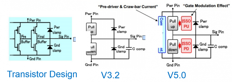
The four IV curve data: pull-up, pull-down, power clamp and ground clamp act like non-linear resistors. With terminal voltage known within each Newton iteration, the conductance can be look-up from these curve tables and obtained using linear interpolation.

The switching coefficients and composite currents are both time dependent. Their values are calculated in the “modeling” phase when simulation has not even started. The obtained coefficients is a multiplier which will further scale the conductance calculated for IV data and thus stamped value. These scaling are such that when test load specified in the waveform section is connected, driver at the pin will reproduce exactly the same waveform data given in the model. As to C-Comp, it can be inserted using simulator’s existing infrastructure so the integrator there will manage the stamping and error prediction.

The more complicated portion of IBIS modeling inside a simulator is due to the options available for the end user, thus model developer must plan in advance. For example, the c_comp may be split across different terminals. Each waveform, IV or components have different skews which book-keeping codes must take care of. There might be added submodel for pre-emphasis or de-emphasis so the class implementation-wise one should consider “composite” pattern such that recursive inclusion can happen. At the end, this is a relative simple device to model for simulator, particular when comparing to the transmission line.

 

W-Element… Transmission line:

Every electromagnetic text book will give transmission line structure as shown below:

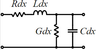
This is an uniform distributed model and is implemented early in various simulators as  the “U” element. While implements T-Line model this way is now outdated due to the performance issue, it’s still how the T-Line’s raw data, frequency dependent tabular model, are given:

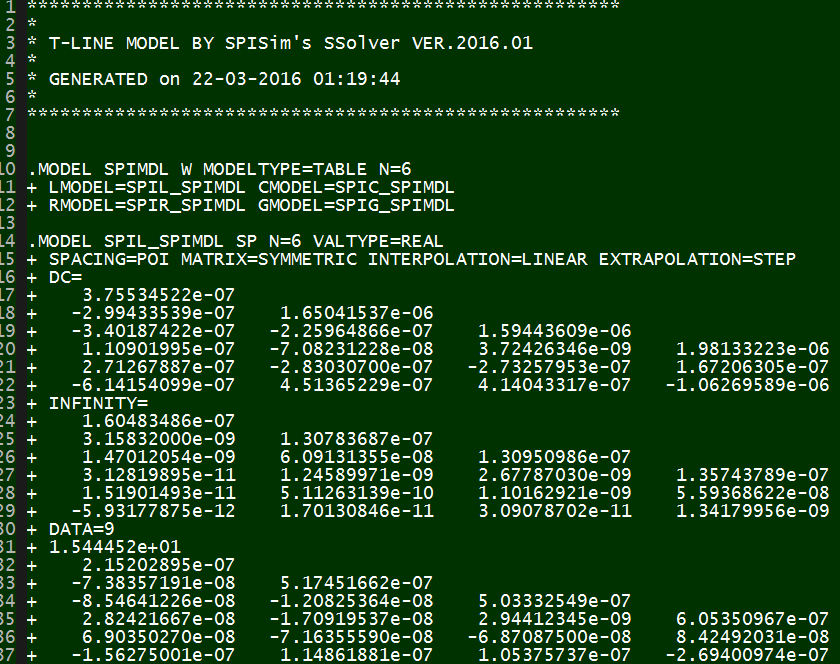
The tabular model are field solved of Maxwell’s equations based on layer stackup, trace layout, material properties and sometime special treatment (like surface roughness) and finally presented as R/L/G/C data at low (DC), high (Infinity) frequencies and many points in between. Thus to model T-Line for a simulator to use, one has to convert these data to a mathematical form first which can then be used in either time or frequency domain. For transmission line, this can starts with Telegrapher’s equations.

By solving the KCL/KVL of a unit length RLGC circuit above, one can derive and find the telegrapher’s equation:

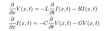
And the solution to this equations, as explained in the wiki link above, involve a wave propagation function Gamma:

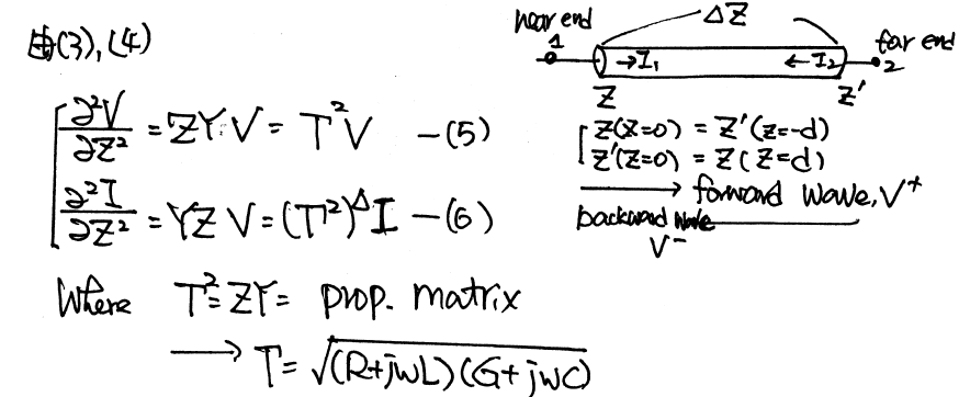
When realize this in the system model, it as the Norton equivalent circuit form:

So on each side (near end and far end) of the transmission line, there are two components: Z (admittance) at that particular time step and current source due to the propagation delay originated from the other end. These two components (Z(s) and r(s)) can be obtained from the tabular data in frequency domain and then converted to integrate-able form in time domain so that they can be “stamped”. Generally, it includes the following steps:

• Parse and store the raw tabular model;
• Calculate the propagation delay and characteristic impedance using highest frequency data (or using extrapolation), these value will be used for interpolation later in time domain.
• Construct the Z(s) or Y(s) and the wave function r(s) shown in the system model. As transmission lines are usually coupled, these curves are multi-dimensional in frequency domain;
• Using vector fitting technique to represent this frequency domain functions using series of poles and zeros. In most of the cases, particular when the model data has insufficient bandwidth or low quality, exact fit is not possible with reasonable number of poles/zeros and thus best fit in the minimum-square-error sense needs to be performed.
• Once pole and zeros are found, they can be converted into time domain as different order of terms. All these terms combined together will form the Y(t) or r(t) in time domain. Pade’s approximation may be used here.
• During time domain simulation, use interpolation to find r(t)’s value in the past history (propagation delay ago) and use that data to construct the equivalent model of this end at this particular time point.
• For frequency domain analysis, vector fitting and conversion to integral form is not needed. The Y(s) and r(s) data can be used directly for stamping at this frequency with some interpolation.

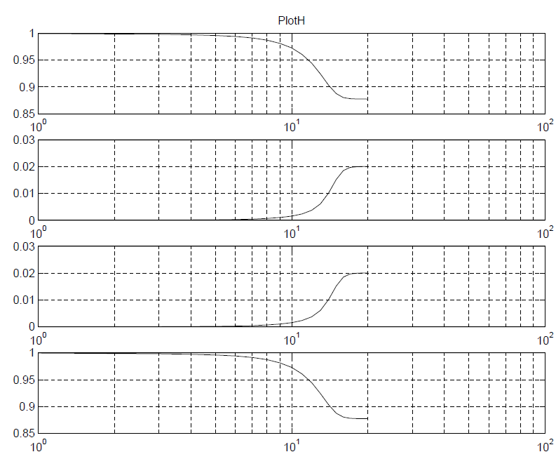
For the first three steps, I wrote a simple matlab codes to demonstrate how how they are done:

Impedance function: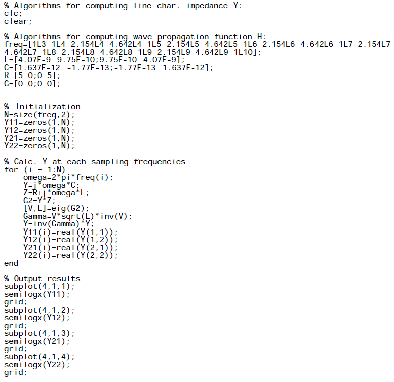

Propagation function: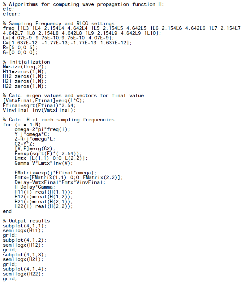

Plots: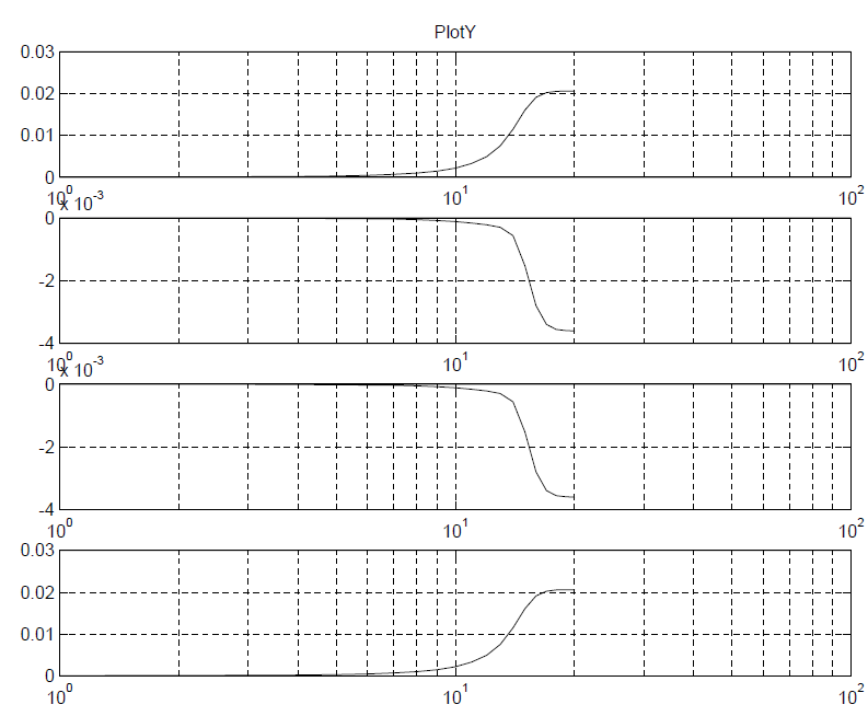

While the matlab codes above seems straightforward,  most simulator (including SPISim’s SSolver) will program with native codes (C/C++) for performance consideration. So a whole lots of matrix operation (inverse, eigen value, LU decomposition etc) will also come into play during the process.

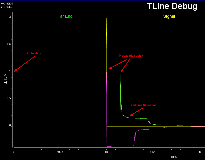
It’s rarely the case that the developed model or codes will work the first try. With so many terms (of converted poles and zeros) for so many dimensions (coupled cases), it’s a daunting task to figure out what has gone wrong when waveform is not as expected. It’s often simpler to back to basic: check steady state solution first, use one line, no reflection with by matching impedance at the other end, use characteristic impedance to find nominal reflection value and so on to help identifying the issue:

Interested reader may find more details about SPISim’s implementation, same as HSpice’s, in the following paper:

“Optimal Transient Simulation of Transmission Lines” by Dmitri Borisovich Kuznetsov, Jose E. Schutt-Aine, IEEE Trans. on Circuit and Systems, I Feb. 1996

In terms of book, I have found that Chap. 5 of Dan Oh’s “High-speed Signaling” book, S6 in our reference book section, give best explanations among others. This maybe because Mr. Oh is from UIUC around the same time when the paper was published as well 🙂 It also worth mentioning that similar technique can be applied to other passive, homogeneous device modeling, such as the system channel. For example,  one common approach of checking and fixing casual issue of a s-parameter is by using vector fitting and convert to rational function form.