Effective analysis methodologies and streamlined flows are built on top of core technologies. For system electrical analysis, these core technologies are mostly 2D/3D field solvers, circuit simulator and statistical processing engine. So far as simulator is concerned, HSpice by Synopsis is often considered as a golden reference. While it is more accessible for us in this part of the world, apparently it may not be the case for other areas, particular in Asia. To enable our customers for system analysis not bounded by the availability of HSpice, we embarked the journey of simulator development last year. As it comes to fruition with the release of SSolver in Q1/2016, we would like to share some of the thought process with the coming posts for readers who interested in how it works. Note that the context here is MNA based electrical simulator, mechanical and thermal etc disciplines are not included.
Circuit simulator is an art of combining computer science, physics and mathematics.
Each junior EE undergraduates learned that circuit analysis, in its most fundamental form, can be done with nodal analysis or mesh analysis. One can use KCL and KVL for the nodal cut-sets and loops in the circuits and form equations representing the circuit’s branch current and nodal voltage.


However, not all of the elements can’t be represented with pure voltage or current form. In order to “probe” voltage or current of particular node or branch, the combined analysis, modified nodal analysis (or MNA), is used. Nodal analysis is used as basis here because there are fewer cut-sets than mesh loops. So when writing all the equations into a matrix form, the dimensions of the matrix for nodal will be considerably smaller and thus more efficient for solving. With the matrix form, it’s thus clear that the circuit analysis is basically linear algebra… store and solving MNA matrix many many times. In my mind, this is where mathematics comes into play. All the matrix’s techniques will apply: sparse matrix, pivoting, conditioning etc. If the matrix is ill conditioned such that after certain iterations, the solutions can’t be found, then simulation does not converge. Is also often an insight simulator designer should place at this stage that how to feedback and relate matrix elements which cause non-convergence back to the original branch so that user may look into the model or connection of that device for further inspections.
While it’s easy to write a program to solve matrix and get a solution vector, it takes a lot more thoughts to do this efficiently during simulation. Without touching device’s physics modeling (yet), this is where knowledge from computer science may be very helpful.
There are many types of circuit analysis: DC, DC Sweep, Transient, AC small signal, Sensitive etc. For system analysis, we probably use transient (time domain) most. However, the most fundamental step for all these are “Newton Iterator“, that is using “Newton Raphson (NR)” technique to solve aforementioned matrix repeatedly until solution vector is found. In DC operating point phase, all models are static (e.g. capacitor is open and inductance is short). Several NR iterations later when DC solution is found, than AC model is used for small signal around this DC operating point or transient model is used to start marching into t > 0 domain. Within each time step, matrix is again consider static (respect to that time step) and many NR iteration will be performed. Nodal voltage will adjust during these iteration as tentative solutions changes, so the model’s physical response must also adjust accordingly. In some cases when DC does not converge, simulator will revert back to “Ramp” or “Charge up” in which all voltage/current sources starts from 0.0 (thus no branch current and nodal voltages are all 0.0), then gradually ramp up the value just like transient simulations.
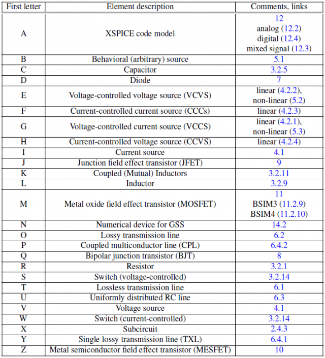
Now there are also many different type of devices (see above), not all of them are non-linear or time varying. So to build an efficient simulator, they need to be architect to minimize function calls and thus matrix element change. For example, one may be able to classify devices into the following several types:
- Not-time varying: e.v. dc source, whose value will not change during simulation
- Time-varying:
- Linear: e.c. PWL source, whose value will not change within that timestep
- Non-linear: transmission lines, whose value will change in each iteration
- Frequency dependent or non-frequency dependent
The purpose of this classification is to make matrix “stamping” (i.e. filling in the value) and solving as efficient as possible. These two steps are the “hot-loop” of the circuit simulation. We can then define device interface:
- Parse: called only once per run, parse the netlist syntax;
- Initialize: once per run, transfer texture data to counterparts for simulation
- Model: before DC starts, construct physical model
- Stamp: depending on device type, called once per simulation, per time step or per iteration
- Solve: called during each iteration to solve for solution vector
- Update: concluded and called at the end of the time step to prep for next time step
- Request: to answer probing request and return device properties
- Cleanup: clean-up the memory at the end of the run.
In objective-oriented language such as C++, these interfaces are realized as virtual functions to be derived and overwrite by the concrete device classes. In language like “C”, they are defined as struct of functional pointers and the derived class must overwrite and called in the same order to avoid pointer mis-alignment. There may be a predefined linklist at the simulator level which has all types of devices involved in the netlist, then simulator iterates each instantiated device within that link list at different time point or iteration to get updated value for NR matrix solving.
Also needs to be considered is the model placement: same models may be shared by many instances, thus it’s not efficient to have model created for each one of the instance. For example, many transistors may use same BSIM model, thus only the first device using this model need to initialize such model structure but not the rest. So at simulator level, separated linked list or hash map needs to be maintained for the model assignment as well.
Other considerations may include varying simulation timestep and new simulation without re-initialization. For the former cases, a predictor is used to predict error may happen if “Jump” to this time step. When actual solving find to much error due to this big jump, than backtracking to smaller time step will happen… so the book-keeping of old matrix should be at hand. Also, most simulator supports “.alter” type statements such that same netlist can be reuse for new simulation with updated device values properties. Thus, the simulator or device designer must make sure that the simulation settings in previous run will not “contaminate” next run.
As one can see, these considerations needs to be think through when designing a circuit simulator. Other wise the developed simulator will easily become unstable and un-maintainable, let alone extensible. On the other hand, it’s also this kind of exercise and process which make a humble engineer appreciate the beauty of different disciplines of science and engineering work flawless to solve modern design and analysis challenges.
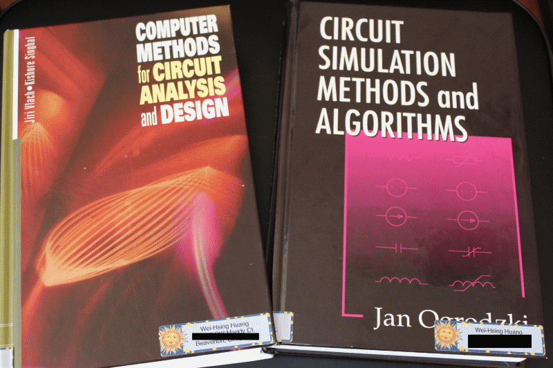
Interested reader can further explore more details in open source simulators such as Berkeley spice, and/or reference to the books recommended below: