

Preface:
This blog post is written in preparation for the upcoming IBIS summits at EPEPS (San Jose, Oct/18/2017), Shanghai (Nov/13/2017) and Taipei (Nov/15/2017), where I will present paper of the same topic. Slides, example models and audio recording will be made available below:
- [MP3 Audio] English, 43 min. Presented at the EPEPS IBIS Summit at San Jose
- [MP3 Audio] Chinese, 45 min. Presented at the Asian IBIS Summit at Taipei
- [Presentation] [Demo files] Both are also available at the IBIS website [HERE]
Motivation:
Many years ago when I entered the signal integrity field, we analyzed the channel by performing spice-like simulation for several hundred nano-seconds at most. Post-process were then done to get FOM metrics. At that time, the bus speed was barely around 1Gbps. These days, high speed-IO SERDEs are common among various computing devices and their speed reaches multi-Gbs or higher easily. Not to mention the several new 802.3 network protocols which have even higher speed (50G~ >100GB). With such high data rate, one needs to “simulate” number of bits at 1E12 level to reach certain bit-error-rate (BER, say 1E-12) with certain confidence level (CI, say 99%) . As such, traditional SI analysis method is no longer valid because it is simply inpossible to simulate so many bits in reasonable time using spice-based simulator. A new channel analysis methodology, like link analysis, is thus needed and invented around year 2003 to address this problem (e.g. StatEye). For link analysis, traditional buffer models such as IBIS are not much useful as they mostly time-domain based. Algorithmic modeling interface (AMI, a subset of IBIS) models are used mostly instead.
AMI modeling is very technically challenging, it requires cross domain expertise such as simulation, modeling and C/C++ programming across different OSes and platforms. Thus it usually takes much longer for an engineer to ramp up to be able to develop and deliver a model when comparing to traditional IBIS. Two of the big hurdles which cause this slow ramp-up for AMI modeling are the requirements to express the circuit’s behaviors in C/C++ language and then be compiled according to Spec’s API requirements. To lower such barriers, we are asked often: 1. Can we create an AMI model using scripting languages? 2. Can I simulate existing spice models using link simulator before committing to develop a full blown C/C++ version?
We propose approaches to meet these two common requests in this presentation.
Background:
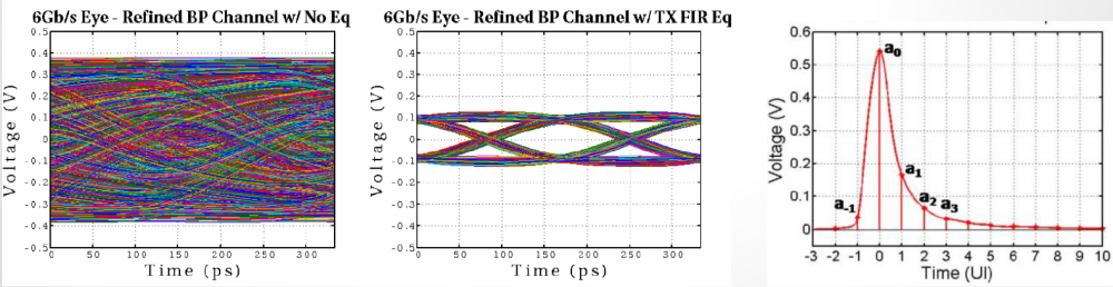
Channel analysis: Nowadays the high speed link analysis most definitely includes stages such as Tx/Rx EQ, which are beyond traditional IBIS. Equalization is needed to compensate channel noise such as inter-symbol interference (self-channel interference) and crosstalk (co-channel interference). These EQ stages can open “eye” from a closed one of a noisy channel, represented by S-parameter interconnect.
There are two analysis methodologies for modern link analysis:
- Statistical: If the circuit is linear time-invariant (LTI), one can obtain many information about channel’s limit by using a single pulse or impulse response. In this flow, a channel is assumed LTI (s-parameter may need to be enforced/fixed in terms of causality, passivity etc first). Its impulse response is then “fed” into Tx/Rx circuitry to obtain the response. By using superimpose (or superposition), response of the channel + circuitry of different UIs are added together and probability of various BER level can be computed from there.
- Bit-by-bit: If a circuit is non-linear time variant (NLTV), then such superposition is not allowed. In that case, a bit-stream may be fed into Tx/Rx circuitry by link tool/simulator to obtain their continuous time-domain response. These outputs are then “convoluted” with LTI channel to obtain overall channel response. In order to do this for many millions of bits, some assumption needs to be made (high-z, to be discussed later) in order to gain speed performance when comparing to same time-domain spice-like nodal analysis. Also, the link tool may break bits to several chunks and feed to Tx/Rx separately before combining them together, with “aliasing” of adjacent chunks of bits being taken care of properly at the link tool level.
AMI models support both of these two channel analysis methodologies.
AMI Model: an IBIS-AMI model contains several parts:
- .ibs file: In the .ibs file, there is a section called “Algorithmic Model” which points to the paths where the .ami and .dll/.so files reside. This keyword block also provides info such as bit, OS platform and the compiler used to generate the .dll/.so files. Other than these info, the .ibs file and AMI model it points to are basically independent. Further more, in the link analysis, traditional IBIS part are often considered “analog front end” and is “absorbed” into either the AMI portion or the channel portion of the data.
- .dll/.so file: This is compiled binary format. The language MUST be plain old C and it must be compatible defined AMI API spec. in order to be able to loaded by the link simulator.
- .ami file: This is the plain text file which contains “config. settings” for the binary .dll/.so files. As shown in the picture below, it has two main sections:
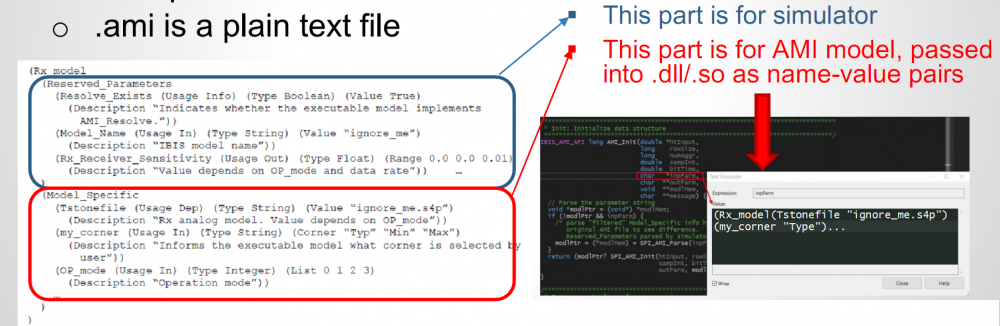
- Reserved Parameters: This block is usually at the top of the .ami file. These settings are for link simulator only. Depending on part of the settings in this block, such as “Resolve_Exists” or “GetWave_Exists” set to true or false, the associated API functions are invoked by the link tool.
- Model Specific: This block is usually at the bottom of the .ami file. It contains AMI model developed defined parameters which link tool and API spec does not interfere with. While there are many “text” in this block, when the .dll/.so portion of the AMI model received their info. passed by the link tool, they have been “filtered” and converted to simple “name-value” pair as shown above. So while the depth of the “tree structure” for this model specific section can have many levels, the parameters received inside the model can be just two levels at its simplest form with model name (RX_model above) at the root and the other name-value pairs as “leaves”.
AMI-API functions: As of IBIS Spec. V6.1, there are up to five API functions can be used in a compiled AMI model:
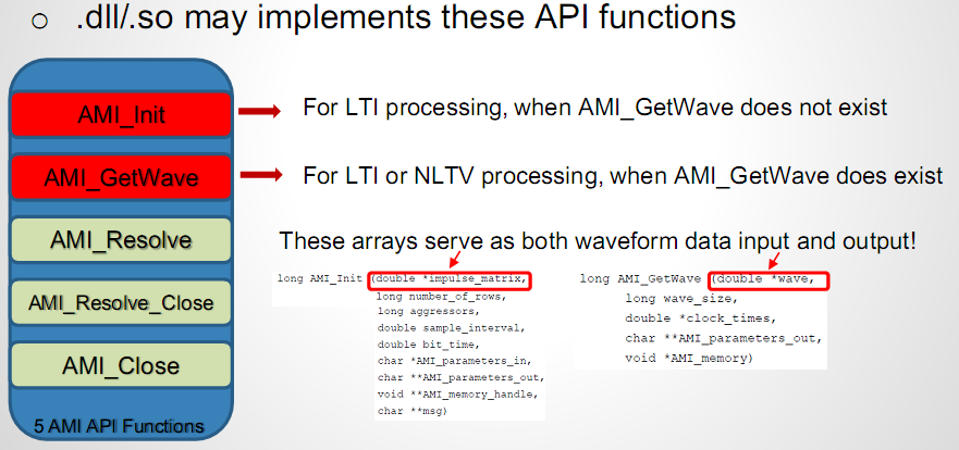
Among which, AMI_Resolve and AMI_Resolve_Close are for string parameter pre-processing which can be ingored in a lot of cases. AMI_Close is like garbage collection/clean-up to release allocated memory, so is trivial is most cases as well. Modern OS may reclaim memory space back even one does not do any “Free” or “Delete” there in AMI_Close. Two most important ones, AMI_Init and AMI_GetWave, are marked in red. In particular, they participate in the aforementioned “Statistical (for LTI)” and “Time-domain bit-by-bit (for NLTV)” models. That is, for a LTI model, its AMI model must/should implement the AMI_Init function call. A LTI model can also implement AMI_GetWave function call but this is optional. On the other hand, a NLTV model must implement AMI_GetWave function while implementing AMI_Init as “initialization” rather than “computing” portion of the codes. The bit-by-bit convolution part of a NLTV model should be implemented in the AMI_GetWave part of the codes.
When looking at the function declaration part of the spec, as boxed in red in right part of the image above, one should also realized that the first arguments (an array represented by double pointer) serves as both input and output purpose. These are “pass by reference” arguments as they are pointer. So at the beginning of the AMI_Init/AMI_GetWave calls, the model can obtain either impulse response of the channel or digital bit sequence from the simulator via this pointer. Then the model perform necessary computing using info from the rest of the arguments (some of them also serve as output purpose, such as char **msg, but is not that important in this context). At the end of the computation of this function call, the modified response must be filled in back to the address where the first arguments points to, so that the link simulator will retrieve the values and carry on the rest of the analysis.
AMI Modeling Flow:
A typical AMI modeling flow involves the following steps:
- Identify the behaviors of circuits being modeled. As we are going to use a computer language to describe the model’s behavior, we must know how it works first. These behaviors can be obtained via either mathematical derivation, simulation results or measurements. In the last two cases, a look-up table may be used inside the model.
- Code the behavior and IBIS-AMI API: There are two parts of this section. The API part MUST be implemented in C (not even C++). The other part of the codes can be in any language, shape or form as long as the developed C codes know how to communicate and exchange the data. That is, the actual computing part, can be in language other than C/C++ if you like or even be completed via circuit simulation.
- Compile and link as .dll/.so: This is the compilation of the strict C portion of the API. In windows, one usually needs to compile for both 32 and 64-bit. On Linux, on top of different bits, one should also test on various distros (debian or red-hat based) as they may use different version of GNU C (and thus support different version of C spec. e.g. C99 (1999) or C11 (2011)
Now let’s talk more about item 2 above. There are many considerations on how you should code this part. A specifically C/C++ coded model for one circuit will mostly run very fast. However, it may requires frequent re-compilation/re-testing when new design comes. If we can make this part as simple as possible and non design specific, such as calling external scripts, then this work may only need to be done once as all the variation are now external to the compiled .dll/.so.
Modeling with Scripts:
Knowing the requirements of the AMI API, we can now propose a flow to create an AMI model using user’s favorite scripting language:
Flow:
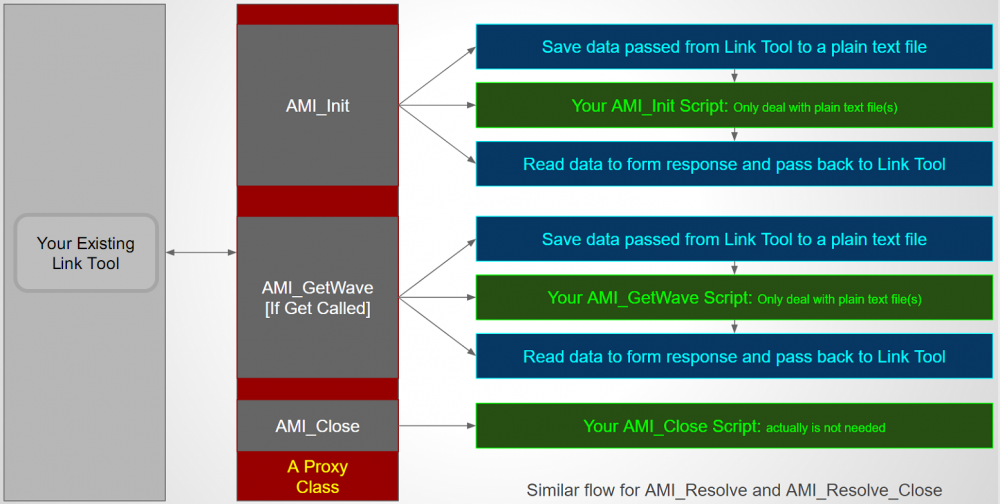
To support script based AMI modeling, we need to have a thin API implementation (in C, as required by AMI Spec) whose sole task is to translate all the received arguments into a text format and write as a text file. It will then pass the path of the text file to user defined scripts or batch file via system call. Location and type of the script is defined in advance in plain-text .ami file. The script needs to retrieve the argument information first by parsing the plain text file, perform necessary computing, then write into another or same text file which this AMI model with thin layer knows where to find. So when the script completes, the AMI model will parse the text file generated by the script, fill the information back to the aforementioned “passed by reference” pointer array, then complete this step. As discussed, whether the scripts is needed for either AMI_Init or AMI_GetWvae or both are pre-defined based on circuit behavior. And since this is developer chosen favorite language, parsing and writing to text file should not be an issue when comparing to say C language. Lastly, should there be any information need to be passed between API calls (such as model member’s values between AMI_Init and AMI_GetWave), they can also be file based. To summarize, the AMI model with thin layer completes the API calls with upper simulator like other regular AMI models. However, its “transactions” with underlying user’s scripts are all file based.
Example:

A matlab example of the AMI_Init is shown above. In the matlab codes, it first calles parseInput function, which is a text file prepared by the thin AMI model and contains input waveform. It then performs computation such as convolve with FFE, then the result matrix is written back to the text file via storeOutput function call which thin AMI model know where to find. Since matlab’s “conv” function is used directly, the model developer does not need to deal with c-based implementation details such as memory allocation FFT/iFFT in some cases or other math library linking/compilation.
Considerations:
While script based AMI development is simple and handy, there are several considerations before deciding to release such models:
- Performance and distributional: Since all communications between thin AMI model and user’s script are file based, it inevitably will suffer some performance issue. If this is AMI_Init, it’s only called once by simulator during analysis and such performance penalty is less of a concern. Next, one must also consider the how the mode can be distributed? If the script is in matlab .m file, then model clients need to have matlab environment installed as well. If it’s in compiled matlab, then client needs to install matlab compiled runtime (MCR). If the scripting language is in perl, then perl interpreter, which is usually installed by default on linux but not Windows, is needed. To distribute such interpreter, one must also check the license terms and then also think about the elegance of such model release.
- Consider Python!: Python is a very worthy candidate here because it has rich math or matlab like libraries such as SciPy or NumPy. More importantly, there is a mechanism called “embedded python” in which the whole python interpreters together with math libraries used can be bundled and distributed in a single zip file. That is, the end user does not need to install python environment first as the thin AMI model already linked with C-Python and can find all required functions in either user’s scripts or bundled zip file.
Modeling with Spice circuits:
Now that we know a thin layer can call external script either directly or via its interpreter, we may also come to the conclusion that it can also call external program such as a circuit simulator. This is of course true!.
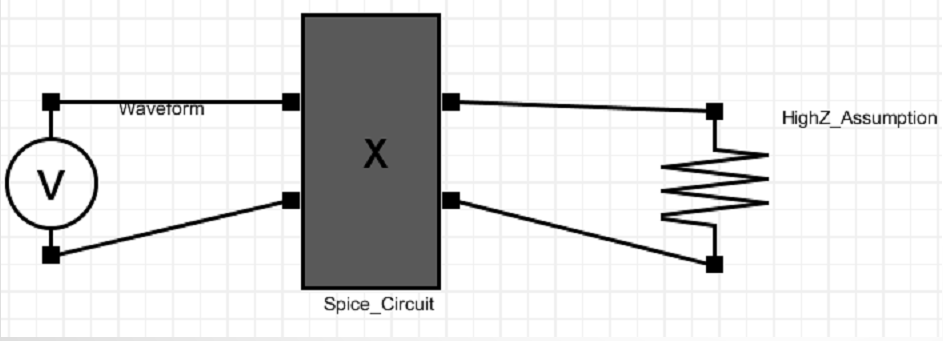
An assumption we mentioned at the beginning of the post is the “High-Z” condition. In a typical spice-like nodal analysis, there are many “Newton-Raphson” iteration going on within same time step. At the beginning of each Newton iteration, tentative voltages are given at each node. Each components then compute the drawing or output current into these nodes based on these voltages and its own behaviors. At the end of the iteration, circuit simulator solves the system matrix to see whether KCL/KVL reaches balance and then determine either another Newton iteration is needed or it can march into next time step.
In channel simulation, such iteration is not needed as there is a “High-Z” assumption… and that’s why it can run much faster than nodal spice simulation. In High-Z assumption, each blocks is assume to have high input impedance and output impedance so it will not draw any current at the input and the output is set once determined. Since the thin layer AMI model can obtain the inputs from simulator via API call, if it can perform another task… such as convert this inputs input PWL source with time step equal to UI/number_sample_per_UI (both are know and passed by the simulator), then it can theoretically call a simulator to drive user provided spice subckt like above. Note that the input waveform is just voltage which represents potential difference of two nodes. So there is no reference to GND at all. It’s subject to user’s spice circuit to determine what the reference is and provide GND reference if needed.
Flow:
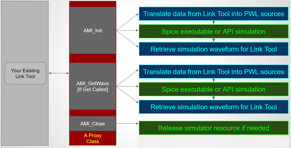
The picture above shows the flow to simulate/model AMI with spice subcircuit. It is very similar to the flow for AMi with scripting language. First the thin layer AMI model need to generate a PWL source dynamically based on the provided inputs. Then form (either write out as a file or internally in memory) a netlist as a driving circuit and probe at the output. This driving circuit will use user provided spice subckt with possible value overrides defined at the .ami file. Then thin layer AMI will call external spice simulator (or internal API) to perform nodal based simulation. The output (like .tr0 for HSpice) is then processed and its value is again filled back to the initial API pointer array to return back to upper circuit simulator.
Example:
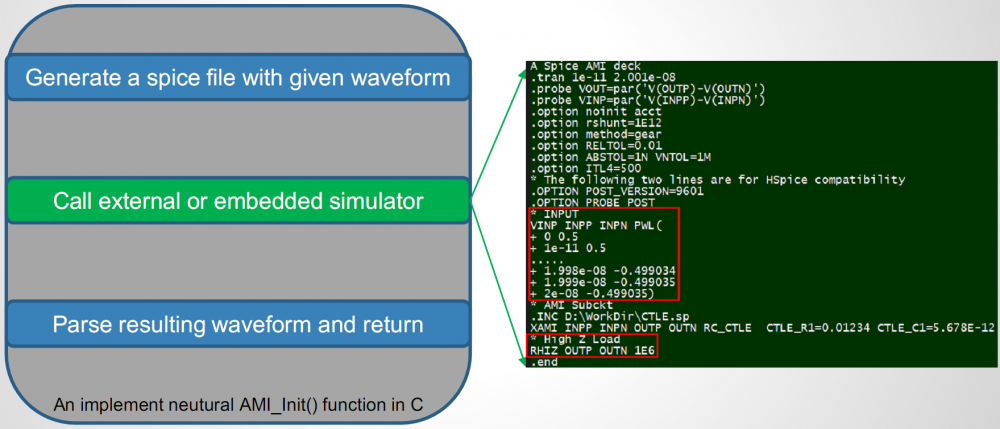
An example is shown above. The template is pre-defined with the PWL source and path to user’s spice circuit being left to be filled-in. The thin AMI generates the netlist with all values filled properly upon being called by simulator. It then call external simulator to do nodal simulation. Resulting waveform are post-processed and filled-in to the API argument memory address and complete this API call.
Considerations:
Similar to the AMI modeling with script language case, there are several considerations when adopting the spice-based AMI modeling approach. First is the performance… as each AMI API call involves nodal simulator initialization (allocate matrix, solve for DC, Newton iteration between each time sample etc), it will be significantly slower than pure C implementation. However, this is less of a concern if only AMI_Init is needed as it’s called only once. More over, one does not need derive any equation or do any coding at all and can get accurate link performance using this Tx/Rx circuitry directly… so development time is saved significantly there. If one decides to implement such block in C/C++, then simulation results obtained during this process can serve as a very good reference or correlation data for C/C++ based model to be developed.
Another consideration is again the distribuability: If this spice model has particular MOSFET model and requires say HSpice, then the AMI model recipient also needs to have HSpice in their environment in order to run. While commercial simulator like HSpice may not provide API or serve as shared library, many open source ones do. Examples are NgSpice and/or QUCS. In these case, the compiled thin AMI model is basically a simulator in .dll/.so form and can perform simulation all by itself. The binary size is around 8MB larger then without as it also needs to link with all simulator supported device models as well.
Summary:
Using either scripts or existing spice circuits for AMI modeling is actually doable. The presentation I give here is not just talk on paper. The implemented “thin-layer AMI” and examples are also provided together with the slides. These flows can be considered as part of the AMI development process as they can shorten the modeling cycle significantly while providing data for correlation should one decide to go full C/C++ implementation at the later stage. The consideration points includes performance, elegance of released models and distributability of either the script’s interpreter or simulator. Also a thin layer AMI models is needed. This thin layer API is called Proxy model in computing science terms. As a matter of fact, SPISim has implemented such proxy models and made them available for public to use free of charge. [Link Here] Having that said, this API model only needs to be done once as all the model variation are located externally in user scripts/spice models. and thus require no re-compilation when design changes. Nevertheless, these two possible modeling approaches provide an AMI model developer alternative ways to decide on how a model can be developed more efficiently and effectively.